Showing posts with label English Language. Show all posts

Color-Kinematics Duality for nonSUSY Yang-Mills

On Wednesday I delivered my second (and last) presentation for the so-called "Research Skills" course of the MSc. As I anticipated in my first talk, the subject was color-kinematics duality (or more commonly called BCJ duality in this case) at one loop in nonSUSY Yang-Mills; the title follows from the article it was based on:
Color-Kinematics Duality for Pure Yang-Mills and Gravity at One and Two Loops
Zvi Bern, Scott Davies, Tristan Dennen, Yu-tin Huang, Josh Nohle
arXiv:1303.6605 [hep-th]
The article was submitted on 26 Mar 2013 and was last revised 14 Jan 2015, so it's almost fresh from the oven.

These are the slides of my talk:


I basically went through the article, even if not in detail (which I don't claim to fully understand) and just mentioned briefly the two-loop and gravity parts. It took me between around 24 (of 25) minutes to finish the presentation, so it was about right. The relevant minimum background to follow the slides or at least superficially read the article is of course QFT and a little QCD.

In the end I received two interesting questions: for the first I pointed out that the "Yang-Mills squared" prescription does not give pure gravity, as denoted in slide 16 with the state decomposition $\underbrace{(1/2,1/2)}_{\text{gluon}}\otimes
\underbrace{(1/2,1/2)}_{\text{gluon}}=
\underbrace{(1,1)}_{\text{graviton}}\oplus
\underbrace{(1,0)\oplus(0,1)}_{\text{anti-sym tensor}}\oplus\underbrace{(0,0)}_{\text{dilaton}}$. A nice account of this can be found in this presentation by Alexander Ochirov: "Pure gravity amplitudes via color-kinematics duality in the fundamental representation".

Excerpt from A. Ochirov's talk: www2.ph.ed.ac.uk/~aochirov/talks/Nordita2015.pdf

The second was concerned with how color-kinematics arise from a more fundamental -group theory- level. The answer is surely not trivial. The article I used references to this other paper:
The Kinematic Algebra From the Self-Dual Sector
Ricardo Monteiro, Donal O'Connell
arXiv:1105.2565 [hep-th]
which I haven't had the time to read in depth, but it certainly should shed some light into this question.

All this "QCD meets gravity" stuff seems really exciting and it seems to be quite active lately... if I pass my examinations with good marks and do a good job with my dissertation project, I might as well consider pursuing a PhD in a related topic :-)

One year in Edinburgh, string amplitudes and the KLT relations

My second semester at the MSc in Mathematical Physics at the University of Edinburgh is almost done (2 weeks) and I'm getting ready for examinations. The assessment scheme is a pretty tough one: I've attended twelve courses since September -some of which ended up being much harder and workload intense than I thought (e.g. linear analysis, advanced QFT, QCD, Lie groups/algebras, standard model)- and 9 of my examinations will count between 80% and 100% towards my final mark; furthermore, I need an average of above 50% with no more than 3 marks below 50% in order to get the degree.

So yes, it's crazy. And I shouldn't be wasting time writing here I guess, but at least I've started by (kind of) blocking my access to facebook, which is a huge distraction.


It's a bit ironic, but throughout the year I became uninspired to follow the path of mathematical physics and even the academic one (completely the opposite to what I expected). The reasons are varied but I guess I can just put it simply as a feeling of not belonging. It's not that I suddenly found that I don't like mathematical physics, I obviously love it, but considering it a full time job in Academia is a somewhat different matter. I'm still considering the pursuit of a PhD in Quantum Information, though, but I think I'll narrow my options to the U.S/Canada and Mexico, if I decide otherwise, God knows (whatever that means) what I'll end up doing.

In other news, one of the courses I'm taking concerns giving two 25 minute talks related to the dissertation topic that one has chosen. My dissertation will be about the so-called colour-kinematics duality: to design and implement Mathematica code which creates the relevant (loop-level) diagrams, determines the Jacobi relations among them, and allows for these objects to be manipulated.

There is a whole other world -unknown to me until now- about this and the most surprising aspect of this colour-kinematics duality is that it enables to obtain a gravity theory scattering amplitudes very easily as (prop to) the square of a gauge theory amplitudes. This then connects with another set of relations between scattering amplitudes in string theory known as the KLT-relations, which so happen to reduce to this gravity = gauge theory squared relations in the low-energy (point-like) limit.


There are two very nice popular-science level stories about this:
What I did for my first presentation was to talk about string amplitudes and KLT: what does these things mean and how to interpret what the KLT relations are saying. It was a bit of a detour because I won't really be working with string theory, however I wanted to find out at least the basics of where this thing come from. For anyone who knows string theory well, I didn't say anything new and most of the slides are contained merely in the introduction of Superstring Theory by Witten, Green and Schwarz.

For anyone really serious about the topic, this paper looks like a really good review:
Perturbative Gravity and Gauge Theory Relations -- A Review
Thomas Sondergaard
arXiv:1106.0033 [hep-th]
In my second talk I'll look in a bit of a detail (as time allows me to prepare) to colour-kinematics (BCJ duality, the Kleiss-Kuijf relations, the double copy and other such words) and probably I'll share something about it here.

These are my slides about string amplitudes and the KLT relations (handout mode):

MOOCs and Online Lectures: Supersymmetry, Extra Dimensions and the Higgs Boson

I fortunately happened to live during the rise and development of the internet and other information technologies. Now I'm witnessing the proliferation of the so called MOOCS and open access to (under)graduate level courses, which is great. I'd say these type of courses and lectures are presumably the best option for those who want to self-teach themselves, those who want to change fields of study, or to those who want to deepen their understanding in some particular topic.

I've gone through the whole of David Tong's lectures on QFT (mentioned in earlier posts) and part of his lectures on String Theory too; these are great by themselves and the QFT ones have some advantage in that there are YouTube videos available (though -the videos, not the lectures- of poor quality). It seems that a lot of leading universities and their academics are (becoming?) aware of the relevance of making available good quality content to the general public, even if not specially by well organized MOOCs but just by access to online lecture notes.

Here I share two courses which I'm currently following.

First:
Cambridge Lectures on Supersymmetry and Extra Dimensions
Lectures by: Fernando Quevedo. Notes by: Sven Krippendorf and Oliver Schlotterer

These lectures on supersymmetry and extra dimensions are aimed at finishing undergraduate and beginning postgraduate students with a background in quantum field theory and group theory. Basic knowledge in general relativity might be advantageous for the discussion of extra dimensions. This course was taught as a 24+1 lecture course in Part III of the Mathematical Tripos in recent years. The first six chapters give an introduction to supersymmetry in four spacetime dimensions, they fill about two thirds of the lecture notes and are in principle self-contained. The remaining two chapters are devoted to extra spacetime dimensions which are in the end combined with the concept of supersymmetry. Videos from the course lectured in 2006 can be found online at this http URL.
I've gone until §2.2 and I find the lecture notes really easy to follow. The math notation has some weird spaces in the equations, (which are not numbered btw) and there are some occasional seemingly non-relevant errors, like on page 19,
\begin{equation*}{N_\alpha}^\beta(x_\nu\sigma^\nu)_{\beta\dot\gamma}N_{\dot\alpha}^{*\,\dot\gamma}\stackrel{\color{blue}{?}}{=}{\Lambda_\mu}^{\nu}x_\nu\sigma^\mu\end{equation*} where the $\alpha\dot{\alpha}$ subindices on the RHS are missing; it could've been written simply as $Nx_\rho\sigma^{\rho}N^\dagger={\Lambda_\mu}^{\nu}x_\nu\sigma^\mu$ or, emphasizing the components, I guess the RHS should've been ${\Lambda_\mu}^{\nu}x_\nu(\sigma^\mu)_{\alpha\dot\alpha}$. Also, the procedure to get this equation isn't explicitly -or more carefully- written in the notes (it can be worked out knowing the $x_\mu\sigma^\mu$ transformations under both groups and using the fact that they are the same; the ${\Lambda_\mu}^\nu$ appears as something like ${\Lambda_\mu}^\alpha{\Lambda_\alpha}^\nu$).

I have to say I didn't really liked the video lectures and I didn't find them very helpful: minor issues like the one above don't get straightened and most of the time Prof. Quevedo (which is no insignificant name in the field) just transfer the notes to the blackboard. That's kind of understandable, but, as in the issue I mentioned, not seeing "balanced" indices at an equation should hurt one's eyes enough. However, some discussions may be useful and it is at least more dynamical to follow the notes along with the videos (I also confess that the accent of Prof. Quevedo became a little annoying to me after a while; I don't blame him though, because I might have a similar one).

Then, there's this beautiful course about the Higgs Boson by the University of Edinburgh on what they call Open Education:
The Discovery of the Higgs Boson
Should we be excited about the Higgs boson? Find out more about particle physics and understanding the universe.

Educators: Christos Leonidopoulos and Luigi Del Debbio.

(...)
This free online course introduces the theoretical tools needed to appreciate the discovery, and presents the elementary particles that have been discovered at the tiniest scales ever explored. Beginning with basic concepts in classical mechanics, the story unfolds through relativity and quantum mechanics, describing forces, matter and the unification of theories with an understanding driven by the tools of mathematics.

Narrating the journey through experimental results which led to the discovery in 2012, the course invites you to learn from a team of world-class physicists at Edinburgh University. Learners participate in discussion of the consequences of the Higgs boson, to physics and cosmology, and towards a stronger understanding and new description of the universe.
(...)
The course is meant to be accessible to everyone with high school education. It's already too late to register formally, but there's also a YouTube playlist available from the previous year's course:


So I guess that's pretty much enough ;-) I've seen a few videos and of course there's a lot of detail you won't see, but at least the big picture is there (I didn't truly realize some things, like how to read the plot of the data) and it is fantastic.

I also like to brag a little because most probably I'll be attending the MSc in Mathematical Physics at Edinburgh ;-)

Visualization of the future building of the Higgs Centre for Theoretical Physics at Edinburgh
(due to open in 2016)

The Dirac action for p-branes from the Polyakov-type action

I still have around half a year off until I start attending my Master's courses (at least if everything, e.g. funding, etc... comes ok), so now I'm trying to follow the String Theory lectures by David Tong. As with the QFT ones, these too are great as an introductory reading at a graduate level or for self-study. Solutions to the example sheets are available from a PhD student named Chris Blair; in particular, here for the first one. What I'm concerned about is problem 2.
The p-brane of me got the joke a little late
(hurdles of a non-native speaker)

In part b, one is asked to
Show that the Dirac action
\begin{equation}S_\text{Dirac}=-T\int{d}^{p+1}\sigma\sqrt{-\det\gamma}\end{equation} where $\sigma^\alpha$, $\alpha=0,\ldots,p$ are coordinates on the brane world-volume and $\gamma_{\alpha\beta}$ is the pullback of the Minkowski metric onto the brane,
\begin{equation}\gamma_{\alpha\beta}=\frac{\p{X}^\mu}{\p\sigma^\alpha}\frac{\p{X}^\nu}{\p\sigma^\beta}\eta_{\mu\nu}\end{equation} is equivalent to the Polyakov-type action with dynamical world-volume metric $g_{\alpha\beta}$,
\begin{equation}S=-\frac{T}{2}\int{d}^{p+1}\sigma\sqrt{-g}\left(g^{\alpha\beta}\p_\alpha{X}^\mu\p_\beta{X}^\nu\eta_{\mu\nu}-(p-1)\right)\label{poly1}\end{equation}

Now, the thing is that in the solution by Blair, he starts off with (\ref{poly1}) replacing the $g$'s by $\gamma$'s, which doesn't seem to be what is asked for. This confused me badly, but finally I managed to see what's going on.

What needs to be done is similar to what is done in part a of the problem. As with the string case, $g_{\alpha\beta}$ is now a new field that is fixed by its own equations of motion. First, let's write (\ref{poly1}) as
\begin{equation}S=-\frac{T}{2}\int{d}^{p+1}\sigma\sqrt{-g}\left(g^{\alpha\beta}\gamma_{\alpha\beta}-(p-1)\right)\label{poly12}\end{equation} so that it can be handled more easily (also, from here it's evident that Blair's approach does not solves the problem). To get the equations of motion for $g_{\alpha\beta}$, we should vary the action, where it's needed the fact that
\begin{equation}\delta\sqrt{-g}=-\frac{1}{2}\sqrt{-g}\,g_{\alpha\beta}\delta{g}^{\alpha\beta}\end{equation} which can be obtained through
\begin{equation}\delta\det{M}=\det{M}\,\text{Tr}\left(M^{-1}\delta{M}\right)\end{equation} namely, Jacobi's formula for invertible $M$ (which here is $g_{\alpha\beta}$, i.e. $\delta{g}=g\,g^{\alpha\beta}\delta{g}_{\alpha\beta}$). Using this, and stationary action $\delta{S}=0$, the equations of motion are
\begin{equation}-\frac{1}{2}g_{\alpha\beta}\left(g^{\rho\sigma}\gamma_{\rho\sigma}-(p-1)\right)+\gamma_{\alpha\beta}=0\end{equation} so that $g_{\alpha\beta}$ is related to $\gamma_{\alpha\beta}$ as
\begin{equation}g_{\alpha\beta}=\frac{2\gamma_{\alpha\beta}}{g^{\rho\sigma}\gamma_{\rho\sigma}-(p-1)}\label{poly2}\end{equation} which is basically eq. (1.25) in the lecture notes for $p=1$, as expected. Now, to finally recover the Dirac action from here, just take the determinant on both sides of (\ref{poly2}), so that
\begin{equation}\sqrt{-g}=\frac{2\sqrt{-\gamma}}{g^{\rho\sigma}\gamma_{\rho\sigma}-(p-1)}\end{equation} and as the $\rho$ and $\sigma$ indices in the denominator are dummy, inserting this in (\ref{poly12}),
\begin{equation}S\bigg|_{\text{EOM}}=-T\int{d}^{p+1}\sigma\sqrt{-\det\gamma}=S_\text{Dirac}\end{equation} which is the actual desired result. Now, of course if $g_{\mu\nu}=\gamma_{\mu\nu}$ the result follows as the conformal factor is simply equal to one and it can be readily used that $\gamma^{\mu\nu}\gamma_{\mu\nu}=p+1$ on (\ref{poly12}) to get the result; however, that apparent solution can get misleading because one can think that the Dirac action is recovered only when $g_{\mu\nu}=\gamma_{\mu\nu}$. The relevant thing of this example is to see that once this new field satisfy it's equations of motion, the original Dirac (or Nambu-Goto) action is recovered. Also one should be able to see what gauge symmetry this new field brings upon, as the equations of motion for $X^\mu$ are the same: for the string it is Weyl invariance, however, I couldn't find the case for the $p$-brane but I guess it should be an analogous conformal symmetry (for now I can only say in page 58 it's stated that a $U(1)$ gauge field $A_\mu$ lives on a D-brane, however, the group language still seems a bit foreign to me ;-)

It seems funny, but in the end all of (super)string theory boils down (the history is quite interesting, from scattering amplitudes to the superstring revolutions to today) to the naive step from relativistic points to strings to branes / worldline to worldsheet to worldvolume.

Representations of the Lorentz group are not unitary and the normal ordered angular momentum

I've mentioned earlier (here, in Spanish anyway) that I'm trying to introduce myself to QFT following this set of lecture notes by David Tong. I recently deleted my Physics SE account, but I happened to note that the mentioned set of lecture notes have become somewhat popular (in a good way), so hopefully someone else than me will find this useful.

First (I'll actually go backwards), in Section 4.1.1 it's stated that, in general, the representation of the Lorentz group $S[\Lambda]$ is not unitary, being that by the definition
\begin{equation}S[\Lambda]=\exp\left(\frac{1}{2}\Omega_{\rho\sigma}S^{\rho\sigma}\right)\label{qftlor1}\end{equation} this representation would be unitary if $(S^{\mu\nu})^\dagger=-S^{\mu\nu}$, which is then shown that doesn't hold. Here, basically, $S^{\mu\nu}$ are the basis generators of Lorentz transformations in spinor representation, $\Omega_{\rho\sigma}$ are the elements of an antisymmetric $4\times4$ matrix that specify the Lorentz transformation (a boost by how much speed, a rotation by what angle, etc) and thus $S[\Lambda]$ is the full Lorentz transformation in spinor rep.

I actually ran into trouble trying to prove that $S[\Lambda]$ is unitary if $S^{\mu\nu}$ are anti-hermitian. The thing was that the notation turned really confusing for me. However, it's stressed out that in (\ref{qftlor1}), the thing making $S[\Lambda]$ a matrix is actually $S^{\mu\nu}$, because these are actually $4\times4$ matrices. For it to be clear, if we were to write the components of $S[\Lambda]$, we'd write something as
\begin{equation}S[\Lambda]^{\alpha\beta}=\exp\left[\frac{1}{2}\Omega_{\rho\sigma}S^{\rho\sigma\alpha\beta}\right]\end{equation} This being said, it's actually pretty easy to make the calculation. By definition, $S[\Lambda]$ is unitary if
\begin{equation}S^\dagger[\Lambda]S[\Lambda]=1\label{qftlor2}\end{equation} To compute $S^\dagger[\Lambda]$ we need to simplify something of the form $\left(e^M\right)^\dagger$ with $M$ a $4\times4$ matrix. Of course
\begin{align}\exp(M)^\dagger&=\left(\sum_{k=0}^\infty\frac{M^k}{k!}\right)^\dagger\nonumber\\
&=\sum_{k=0}^\infty\frac{1}{k!}\left(M^k\right)^\dagger\nonumber\\
&=\sum_{k=0}^\infty\frac{1}{k!}\left(M^\dagger\right)^k=\exp\left(M^\dagger\right)\end{align} which seems pretty obvious, but when you don't remember these things by heart (and you shouldn't), it's far better to be sure. This way, the requirement (\ref{qftlor2}) translates into
\begin{equation}\exp\left[\frac{1}{2}\left(\Omega_{\rho\sigma}S^{\rho\sigma}\right)^\dagger+\frac{1}{2}\Omega_{\rho\sigma}S^{\rho\sigma}\right]=1\end{equation} Now, as said before, the matrix is $S^{\mu\nu}$ while $\Omega_{\mu\nu}$ are real numbers, so the expected result follows
\begin{equation}\exp\left[\frac{1}{2}\Omega_{\rho\sigma}\left(\left(S^{\rho\sigma}\right)^\dagger+S^{\rho\sigma}\right)\right]=1\,\Longrightarrow\,\left(S^{\rho\sigma}\right)^\dagger=-S^{\rho\sigma}\end{equation} So, at the end, the calculation was indeed kind of naive. All this beginning of section 4 is probably the part of the lecture notes that has gotten the most of me, mainly because I've got no formal knowledge of Representation Theory nor Lie groups or anything like that, so despite that I find myself flashy with all the new lexicon, I admit I have a long road ahead. A related discussion about non-unitary representations can be found here.
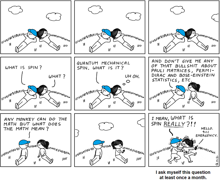
Abstruse Goose - Moment of Clarity
Abstruse Goose - Moment of Clarity 2

The other thing I got stuck with while ago was to compute the angular momentum (this is actually twice angular momentum)
\begin{equation}Q_i\equiv-2\epsilon_{ijk}\int{d^3x}\,x^kT^{0j}\label{qftlorFIN}\end{equation} where ${T^\mu}_\nu=\frac{\partial\mathcal{L}}{\partial(\partial_\mu\phi)}\partial_\nu\phi-{\delta^\mu}_\nu\mathcal{L}$ with the Lagrangian $\mathcal{L}=\frac{1}{2}\partial_\mu\phi\partial^\mu\phi-\frac{1}{2}m^2\phi^2$ on the real scalar field $\phi=\phi(x)$. Basically a Klein-Gordon real scalar. This constitutes problem 7 on Example sheet 2 of the lecture notes by David Tong. I originally posted the question on Physics SE and got no answer before I deleted my profile.

The ultimate issue wasn't really about a mistake, nor about normal ordering. The final expression of $Q_i$ in terms of ladder operators should be
\begin{equation}Q_i=-i\epsilon_{ijk}\int\frac{d^3p}{(2\pi)^3} a^\dagger_\vec{p}\left(p_j\frac{\partial}{\partial{p}^k}-p_k\frac{\partial}{\partial{p}^j}\right) a_\vec{p}\label{qftlorfin}\end{equation} So next I write the whole nasty calculation; if you don't feel like following it all, just skip to eq. (\ref{qftlor5}).

As $T^{0j}=\dot\phi\partial^j\phi$ and
\begin{align}\phi=\int\frac{d^3p}{(2\pi)^3}\frac{1}{\sqrt{2E_\vec{p}}}\left(a_\vec{p} e^{i\vec{p}\cdot\vec{x}}+a^\dagger_\vec{p} e^{-i\vec{p}\cdot\vec{x}}\right)\label{qftlor3}\\\dot\phi=-i\int\frac{d^3p}{(2\pi)^3}\sqrt{\frac{E_\vec{p}}{2}}\left(a_\vec{p} e^{i\vec{p}\cdot\vec{x}}-a^\dagger_\vec{p} e^{-i\vec{p}\cdot\vec{x}}\right)\label{qftlor4}\\\partial^j\phi=-i\int\frac{d^3p}{(2\pi)^3}\frac{p^j}{\sqrt{2E_\vec{p}}}\left(a_\vec{p} e^{i\vec{p}\cdot\vec{x}}-a^\dagger_\vec{p} e^{-i\vec{p}\cdot\vec{x}}\right)\end{align} then
\begin{align}&Q_i=-2\epsilon_{ijk}\int{d^3x}\,x^k\dot\phi_p(x)\partial^j\phi_q(x)\nonumber\\ &=\epsilon_{ijk}\sqrt{\frac{E_\vec{p}}{E_\vec{q}}}\int\frac{d^3pd^3qd^3x}{(2\pi)^6}x^kq^j\left(a_\vec{p}e^{i\vec{p}\cdot\vec{x}}-a^\dagger_\vec{p}e^{-i\vec{p}\cdot\vec{x}}\right)\left(a_\vec{q}e^{i\vec{q}\cdot\vec{x}}-a^\dagger_\vec{q}e^{-i\vec{q}\cdot\vec{x}}\right)\nonumber\\ &=\cdots\left(a_\vec{p}a_\vec{q}e^{i(\vec{p}+\vec{q})\cdot\vec{x}}+a_\vec{p}^{\dagger}a_\vec{q}^{\dagger}e^{-i(\vec{p}+\vec{q})\cdot\vec{x}}-a_\vec{p}a^\dagger_\vec{q}e^{i(\vec{p}-\vec{q})\cdot\vec{x}}-a^\dagger_\vec{p}a_\vec{q}e^{-i(\vec{p}-\vec{q})\cdot\vec{x}}\right)\end{align} Now,
\begin{align}\int{d^3x}\,x^ke^{i(\vec{p}\pm\vec{q})\cdot\vec{x}}=\mp{i}\frac{\partial}{\partial{p}^k}\int{d^3x}\,e^{i(\vec{p}\pm\vec{q})\cdot\vec{x}}=\mp{i}\,(2\pi)^3\frac{\partial}{\partial{p}^k}\delta(\vec{p}\pm\vec{q})\end{align} and so
\begin{align}Q_i=-i\epsilon_{ijk}&\sqrt{\frac{E_\vec{p}}{E_\vec{q}}}\int\frac{d^3pd^3q}{(2\pi)^3}q^j\left[(a_\vec{p}a_\vec{q}-a^\dagger_\vec{p}a^\dagger_\vec{q})\frac{\partial}{\partial{q}^k}\delta(\vec{p}+\vec{q})+(a_\vec{p}a^\dagger_\vec{q}-a^\dagger_\vec{p}a_\vec{q})\frac{\partial}{\partial{q}^k}\delta(\vec{p}-\vec{q})\right]\end{align} Now, integrating by parts on $q$, for example, for the first term
\begin{align}\epsilon_{ijk}a_\vec{p}\int{d^3q}\,q^ja_\vec{q}\frac{\partial}{\partial{q}^k}\delta(\vec{p}+\vec{q})&=-\epsilon_{ijk}a_\vec{p}\int{d^3q}\,q^j\left[\frac{\partial}{\partial{q}^k}a_\vec{q}\right]\delta(\vec{p}+\vec{q})\nonumber\\ &=\epsilon_{ijk}a_\vec{p}p^j\frac{\partial}{\partial(-p)^k}a_{-\vec{p}}\end{align} Then, integrating each term in $q$,
\begin{align}Q_i=-i\epsilon_{ijk}&\int\frac{d^3p}{(2\pi)^3}p^j\left[a_\vec{p}\frac{\partial}{\partial(-p)^k}a_{-\vec{p}}-a^\dagger_\vec{p}\frac{\partial}{\partial(-p)^k}a^\dagger_{-\vec{p}}-a_\vec{p}\frac{\partial}{\partial{p}^k}a^\dagger_\vec{p}+a^\dagger_\vec{p}\frac{\partial}{\partial{p}^k}a_\vec{p}\right]\end{align} The first two terms vanish upon integration because they are odd in $p$, leaving
\begin{equation}Q_i=-i\epsilon_{ijk}\int\frac{d^3p}{(2\pi)^3}p^j\left[a^\dagger_\vec{p}\frac{\partial}{\partial{p}^k}a_\vec{p}-a_\vec{p}\frac{\partial}{\partial{p}^k}a^\dagger_\vec{p}\right]\label{qftlor5}\end{equation} So, finally comes normal ordering.

I was skeptical at first but the calculation goes well step-by-step and the pieces seem to fit together well. The normal ordering is
\begin{align}:a^\dagger_\vec{p}(\partial_ka_\vec{p})-a_\vec{p}(\partial_ka^\dagger_\vec{p}):&=a^\dagger_\vec{p}(\partial_ka_\vec{p})-:a_\vec{p}(\partial_ka^\dagger_\vec{p}):\nonumber\\ &=a^\dagger_\vec{p}(\partial_ka_\vec{p})-(\partial_ka^\dagger_\vec{p})a_\vec{p}\nonumber\\ &=2a^\dagger_\vec{p}(\partial_ka_\vec{p})-\partial_k(a^\dagger_\vec{p}a_\vec{p})\label{qftlorf2}\end{align} (where of course I'm using $\partial_k=\frac{\partial}{\partial{p}^k}$) which yields the correct answer if $\partial_k(a^\dagger_\vec{p}a_\vec{p})=0$. I also noticed that $\partial_k(a^\dagger_\vec{p}a_\vec{p})=\partial_k(a_\vec{p}a^\dagger_\vec{p})$ since
\begin{equation}[a_\vec{p},a^\dagger_\vec{p}]=(2\pi)^3\delta(0)\label{qftL1}\end{equation}
After that long, burdensome and nasty calculation, I was unable to show that indeed $\partial_k(a^\dagger_\vec{p}a_\vec{p})=0$. I recently managed to do so and it goes as follows.

Knowing that $\partial_k(a^\dagger_\vec{p}a_\vec{p})=a_\vec{p}^\dagger(\partial_ka_\vec{p})+(\partial_ka^\dagger_\vec{p})a_\vec{p}$, one can proceed by inverting the Fourier transforms (\ref{qftlor3}) and (\ref{qftlor4}), getting a sum and a substraction of $a_\vec{p}$ and $a_\vec{p}^\dagger$, which can be combined to yield
\begin{align}a_\vec{p}&=\int{d^3x}\,f(x)\,e^{-i\vec{p}\cdot\vec{x}}\label{qftlorf8}\\
a_\vec{p}^\dagger&=\int{d^3y}\,g(y)\,e^{i\vec{p}\cdot\vec{y}}\label{qftlorf9}\end{align} with $f=\alpha\phi+\beta\dot\phi$ and $g=\alpha\phi-\beta\dot\phi$ (keep in mind that these are the operators), and thus,
\begin{align}a_\vec{p}^\dagger(\p_ka_\vec{p})&=-i\int{d^3x\,d^3y}\,x^kg(y)f(x)e^{-i\vec{p}\cdot(\vec{x}-\vec{y})}\\
(\p_ka_\vec{p}^\dagger)a_\vec{p}&=i\int{d^3x\,d^3y}\,y^kg(y)f(x)e^{-i\vec{p}\cdot(\vec{x}-\vec{y})}\end{align} so that, being $x$, $y$ integration variables, indeed,
\begin{equation}\partial_k(a^\dagger_\vec{p}a_\vec{p})=a_\vec{p}^\dagger(\partial_ka_\vec{p})+(\partial_ka^\dagger_\vec{p})a_\vec{p}=0\end{equation} Also, however, knowing the final result from the start, one could have expect from (\ref{qftlor5}), and then show in a similar fashion, that $a_\vec{p}^\dagger(\partial_ka_\vec{p})=-a_\vec{p}(\partial_ka^\dagger_\vec{p})+\delta(0)$, just to finally do the normal ordering and remove the $\delta(0)$ infinity, which arises from $[f(x),g(y)]\propto\delta(x-y)$. It all just falls into place, so normal ordering does not seem to have been the problem either: I guess I was just being plain lazy because I didn't expected to need (\ref{qftlorf8}) and (\ref{qftlorf9}).

So finally, (\ref{qftlor5}) turns into
\begin{equation}Q_i=-2i\epsilon_{ijk}\int\frac{d^3p}{(2\pi)^3}\,a^\dagger_\vec{p}\left(p^j\frac{\partial}{\partial{p}^k}\right)a_\vec{p}\end{equation} which is equivalent to (\ref{qftlorFIN}); however, this is the antisymmetric $\epsilon_{ijk}$ times something symmetric, so the whole thing is antisymmetric and can be written as $-\epsilon_{ijk}\int{d^3x}\left(x^kT^{0j}-x^jT^{0k}\right)$. This way the result written as (\ref{qftlorfin}) follows. As said before, this is actually twice the actual angular momentum operator, so I'll just drop the $2$ factor.

So let's try the new toy: being $|\vec{p}\rangle=a_\vec{p}^\dagger|0\rangle$ the one-particle state with momentum $\vec{p}$, using the relation (\ref{qftL1}) and integrating by parts, we find
\begin{align}Q_i|\vec{p}\rangle&=-i\epsilon_{ijk}\int\frac{d^3q}{(2\pi)^3}\,a^\dagger_\vec{q}\left(q^j\frac{\partial}{\partial{q}^k}\right)a_\vec{q}a_\vec{p}^\dagger|0\rangle\nonumber\\
&=-i\epsilon_{ijk}\int\frac{d^3q}{(2\pi)^3}\,a^\dagger_\vec{q}\left(q^j\frac{\partial}{\partial{q}^k}\right)\delta(\vec{p}-\vec{q})|0\rangle\nonumber\\
&=i\epsilon_{ijk}\int{d^3q}\,q^j\delta(\vec{p}-\vec{q})\frac{\partial}{\partial{q}^k}a_\vec{q}^\dagger|0\rangle\nonumber\\
&=i\epsilon_{ijk}p^j\frac{\partial}{\partial{p}^k}|\vec{p}\rangle\end{align} And one can readily see with (\ref{qftlorf9}) that a one particle state with no momentum, $|\vec{p}=\vec{0}\rangle=a_\vec{0}^\dagger|0\rangle$ carries no internal angular momentum or spin, $Q_i|0\rangle=0$, as expected.

Finally, the previous Abstruse Goose cartoon, and the next one, reminded me of this old slogan that a lot of people I've come across preaches:
Sure, I know you can do the math, but do you really understand it?

In physics there's always this thing about understanding results physically, and that's fine, but a lot of people seem to read this as ultimately reduce all mathematical results to apples and oranges. A discussion about the first cartoon can be found here, and as can be seen, there's no problem whatsoever for people to understand things physically without reducing them to potatoes (which, when done, happens at a price, as science communicators know). To develop an intuition about physical phenomena is, however, a different matter, but then again, one that's mainly driven mathematically.
Our experience up to date justifies us in feeling sure that in Nature is actualized the ideal of mathematical simplicity. It is my conviction that pure mathematical construction enables us to discover the concepts and the laws connecting them which give us the key to the understanding of the phenomena of Nature. Experience can of course guide us in our choice of serviceable mathematical concepts; it cannot possibly be the source from which they are derived; experience of course remains the sole criterion of the serviceability of a mathematical construction for physics, but the truly creative principle resides in mathematics. In a certain sense, therefore, I hold it to be true that pure thought is competent to comprehend the real, as the ancients dreamed.

—A. Einstein, “On the Method of Theoretical Physics

Of course there is still a great deal to learn for us all, and wandering moments remain essential to accomplish that ;-)

Abstruse Goose - Moment of Clarity
Abstruse Goose - Moment of Clarity 1

Null geodesics and affine parameters

I've been away for a while preparing my IELTS test and I hope I'll be ok, whatever my fate is! So, concerning this entry, it came to mind this Physics SE answer I wrote some time ago, where the original poster commented he was only concerned with proper time. In turn I posted this link to another Physics SE answer which deals with what an affine parameter is.

So, the thing is pretty straightforward: the definition of proper time is just the arc length
\begin{equation}\tau=\int\sqrt{-ds^2}\end{equation} and for null geodesics, (by definition) $ds^2=0$, so that's why "proper time assigns the same value to all points (on a null) geodesic". For spacelike and timelike geodesics, $ds^2\neq0$ and $\dot{s}^2=\pm1$ when proper time is the parameter.

Now, recall the geodesic equations for a curve $x=x(\lambda)$ on an arbitrary parameter $\lambda$ with a tangent vector $U\equiv\frac{dx}{d\lambda}$,
\begin{equation}\left(\frac{dU}{d\lambda}\right)^\alpha=\frac{d^2x^\alpha}{d\lambda^2}+\frac{dx^\beta}{d\lambda}\frac{dx^\mu}{d\lambda}{\Gamma^\alpha}_{\mu\beta}=0\end{equation} usually written shorthand as
\begin{equation}(\nabla_{U}{U})^\alpha\equiv{U}^\beta\nabla_\beta{U}^\alpha=0\label{dagger}\end{equation}
So, let's now consider another arbitrary parameter ${\sigma=\sigma(\lambda)}$. Then,
\begin{align}\frac{d}{d\lambda}&=\frac{d\sigma}{d\lambda}\frac{d}{d\sigma}\nonumber\\[0.2in]
\frac{d^2}{d\lambda^2}&=\left(\frac{d\sigma}{d\lambda}\frac{d}{d\sigma}\right)\left(\frac{d\sigma}{d\lambda}\frac{d}{d\sigma}\right)\nonumber\\&=\frac{d\sigma}{d\lambda}\left[\frac{d}{d\sigma}\left(\frac{d\sigma}{d\lambda}\right)\frac{d}{d\sigma}+\frac{d\sigma}{d\lambda}\frac{d^2}{d\sigma^2}\right]\nonumber\\&=\frac{d\sigma}{d\lambda}\left[\frac{\left(\frac{d^2\sigma}{d\lambda^2}\right)}{\frac{d\sigma}{d\lambda}}\frac{d}{d\sigma}+\frac{d\sigma}{d\lambda}\frac{d^2}{d\sigma^2}\right]\end{align} and the geodesic equations on $\sigma$ are
\begin{equation}\frac{\left(\frac{d^2\sigma}{d\lambda^2}\right)}{\frac{d\sigma}{d\lambda}}\frac{dx^\alpha}{d\sigma}+\frac{d\sigma}{d\lambda}\frac{d^2x^\alpha}{d\sigma^2}+\frac{d\sigma}{d\lambda}\frac{dx^\beta}{d\sigma}\frac{dx^\mu}{d\sigma}{\Gamma^\alpha}_{\mu\beta}=0\end{equation} i.e., from (\ref{dagger}),
\begin{equation}U^\beta\nabla_\beta{U}^\alpha=-\frac{\left(\frac{d^2\sigma}{d\lambda^2}\right)}{\left(\frac{d\sigma}{d\lambda}\right)^2}U^\alpha\end{equation} so that from the start, in principle, one could've defined the geodesic equations as ${\nabla_UU\propto{U}}$; however, if
\begin{equation}\frac{d^2\sigma}{d\lambda^2}=0\,\,\Longrightarrow\,\,\sigma=a\lambda+b\label{ddagger}\end{equation} (\ref{dagger}) is recovered. These $\sigma$'s are called affine parameters, and this is why they have this simple form.

Now, (I think) this is where trouble comes. Some authors, e.g. Carroll, define an affine parameter as any parameter related to the proper time $\tau$ as $\sigma=a\tau+b$. The thing is that also, usually it is said that one should use an affine parameter for null geodesics (as in the previous Physics SE answer I mentioned before), but still with this last definition you end up with a constant parameter. So what is generally understood as an affine parameter is simply that with which (\ref{dagger}) is satisfied. For null geodesics, (\ref{dagger}) is trivially satisfied with $\tau$ (or any linear combination whatsoever) so that this parameter is indeed useless; however one is free to use any affine parameter as defined in (\ref{ddagger}) with non-constant $\lambda\in\mathbb{R}$ regardless of its physical relevance.

Now, the term $\nabla_{U}{U}=\frac{dU}{d\lambda}=\frac{d^2x}{d\lambda^2}$ is indeed the acceleration of an observer along the curve $x=x(\lambda)$, so that when using an affine parameter, the observer is not accelerating, while au contraire, with a non-affine parameter, the observer will be accelerated parallel to the direction of movement. This is the main relevance of this sort of parameter; in General Relativity it's the custom to deal with affine parameters where $\tau$, of course, is our favorite one for timelike geodesics, whereas with null geodesics people usually don't care what the parameter is as long as it works, at the end it's all about a goofy parameter ;-)

I go back to May 1937

by Sharon Olds

I see them standing at the formal gates of their colleges,
I see my father strolling out
under the ochre sandstone arch, the
red tiles glinting like bent
plates of blood behind his head, I
see my mother with a few light books at her hip
standing at the pillar made of tiny bricks,
the wrought-iron gate still open behind her, its
sword-tips aglow in the May air,
they are about to graduate, they are about to get married,
they are kids, they are dumb, all they know is they are
innocent, they would never hurt anybody.
I want to go up to them and say Stop,
don’t do it—she’s the wrong woman,
he’s the wrong man, you are going to do things
you cannot imagine you would ever do,
you are going to do bad things to children,
you are going to suffer in ways you have not heard of,
you are going to want to die. I want to go
up to them there in the late May sunlight and say it,
her hungry pretty face turning to me,
her pitiful beautiful untouched body,
his arrogant handsome face turning to me,
his pitiful beautiful untouched body,
but I don’t do it. I want to live. I
take them up like the male and female
paper dolls and bang them together
at the hips, like chips of flint, as if to
strike sparks from them, I say
Do what you are going to do, and I will tell about it.

Wise Men In Their Bad Hours

by Robinson Jeffers

Wise men in their bad hours have envied
The little people making merry like grasshoppers
In spots of sunlight, hardly thinking
Backward but never forward, and if they somehow
Take hold upon the future they do it
Half asleep, with the tools of generation
Foolishly reduplicating
Folly in thirty-year periods; the eat and laugh too,
Groan against labors, wars and partings,
Dance, talk, dress and undress; wise men have pretended
The summer insects enviable;
One must indulge the wise in moments of mockery.
Strength and desire possess the future,
The breed of the grasshopper shrills, "What does the future
Matter, we shall be dead?" Ah, grasshoppers,
Death's a fierce meadowlark: but to die having made
Something more equal to the centuries
Than muscle and bone, is mostly to shed weakness.
The mountains are dead stone, the people
Admire or hate their stature, their insolent quietness,
The mountains are not softened nor troubled
And a few dead men's thoughts have the same temper.

The development of the first nuclear bombs

I recently formulated a question on Physics Stack Exchange for which I received a rather illustrious answer. I'd like to share it here, though if you are an active researcher, academic or student of physics, you can always join Physics SE and vote up both the question and the answer ;) . There's also another answer and some comments that you may find informative.

So the question was:
I've just read that 68 years ago Little Boy was dropped on Hiroshima, which made me wonder about some rather historical facts about the development of the first nuclear bombs; they seem to be several questions, but they boil down to the same thing: the theoretical aspects of the development of the bombs.

As far as I know, nuclear fission was already understood at the time, so was all the competition between the american team and the german team to develop the bomb first, a mere matter of engineering? Or what was the role of theoretical physicists such as Richard Feynman? Also, I've heard things like that the team led by Werner Heisenberg had misconceptions about nuclear fission, so that his team could not develop the bomb first.

Can anyone put in perspective the theoretical aspects of the development of the bombs taking care of this historical issues?

And the answer, given by Physics SE user Ben Crowell, goes like this:
Only some very, very basic knowledge about the physics of nuclear fission was available at this time. I'll give a few details about this below. Also, according to this 1967 interview with Heisenberg, it's probably not accurate to imagine a competition between the US and the Nazis to build a bomb; the Germans were struggling to keep fighting at all in Europe, and didn't think it was realistic to produce more than research reactors given the time and resources they had available.

The liquid drop model dated back to 1935, so physicists, even non-specialists like Einstein, could readily understand the basic idea that fission was possible and that it should release neutrons, making a chain reaction possible. However, fission is a tunneling process, and tunneling depends exponentially on the width and height of the barrier, making it extremely difficult, even today, to calculate fission rates from first principles to even order-of-magnitude precision. People today would typically approach this kind of calculation using the Strutinsky smearing technique, which wasn't invented until 1968 (Strutinsky, Nucl. Phys. A122 (1968) 1; described in http://arxiv.org/abs/1004.0079 ). A primitive version of the nuclear shell model had been proposed, but it wasn't until Maria Goeppert-Mayer in the 50's that it was really developed into a detailed theory, and it only worked for spherical nuclei -- uranium and plutonium are deformed. Even gross features of the barrier, like the existence of a metastable minimum (fission isomers), were not to be discovered until the 60's. So induced fission cross-sections and average neutron multiplicities had to be measured empirically:
[W]hile Glenn Seaborg's team had proven in March 1941 that plutonium underwent neutron-induced fission, it was not known yet if plutonium released secondary neutrons during bombardment. Further, the exact sizes of the "cross sections" of various fissionable substances had yet to be determined in experiments using the various particle accelerators then being shipped to Los Alamos. (source)
The Germans also set themselves back because of Heisenberg's decision to use heavy water as a moderator, when graphite would have been easier. This was apparently partly based on a mistake in a 1940 measurement by Bothe.

There have been lots of hints (possibly involving wishful thinking and retroactive rewriting of history) by the German physicists that they may have dragged their feet or intentionally made mistakes, because they didn't want their own country to get the bomb. The true nature of Heisenberg’s role in the Nazi atomic bomb effort is a fascinating question, and dramatic enough to have inspired a well- received 1998 theatrical play, “Copenhagen.” The real story, however, may never be completely unraveled. Heisenberg was the scientific leader of the German bomb program up until its cancellation in 1942, when the German military decided that it was too ambitious a project to undertake in wartime, and too unlikely to produce results. Some historians believe that Heisenberg intentionally delayed and obstructed the project because he secretly did not want the Nazis to get the bomb. Heisenberg’s apologists point out that he never joined the Nazi party, and was not anti-Semitic. He actively resisted the government’s Deutsche-Physik policy of eliminating supposed Jewish influences from physics, and as a result was denounced by the S.S. as a traitor, escaping punishment only because Himmler personally declared him innocent. One strong piece of evidence is a secret message carried to the U.S. in 1941, by one of the last Jews to escape from Berlin, and eventually delivered to the chairman of the Uranium Committee, which was then studying the feasibility of a bomb. The message stated “...that a large number of German physicists are working intensively on the problem of the uranium bomb under the direction of Heisenberg, [and] that Heisenberg himself tries to delay the work as much as possible, fearing the catastrophic results of success. But he cannot help fulfilling the orders given to him, and if the problem can be solved, it will be solved probably in the near future. So he gave the advice to us to hurry up if U.S.A. will not come too late.” The message supports the view that Heisenberg intentionally misled his government about the bomb’s technical feasibility; German Minister of Armaments Albert Speer wrote that he was convinced to drop the project after a 1942 meeting with Heisenberg because “the physicists themselves didn’t want to put too much into it.” Heisenberg also may have warned Danish physicist Niels Bohr personally in September 1941 about the existence of the Nazi bomb effort.

On the other side of the debate, critics of Heisenberg say that he clearly wanted Germany to win the war, that he visited German-occupied territories in a semi-official role, and that he simply may not have been very good at his job directing the bomb project. On a visit to the occupied Netherlands in 1943, he told a colleague, “Democracy cannot develop sufficient energy to rule Europe. There are, therefore, only two alternatives: Germany and Russia. And then a Europe under German leadership would be the lesser evil.” Cassidy 2000 argues that the real point of Heisenberg’s meeting with Bohr was to try to convince the U.S. not to try to build a bomb, so that Germany, possessing a nuclear monopoly, would defeat the Soviets — this was after the June 1941 entry of the U.S.S.R. into the war, but before the December 1941 Pearl Harbor attack brought the U.S. in. Bohr apparently considered Heisenberg’s account of the meeting, published after the war was over, to be inaccurate. The secret 1941 message also has a curious moral passivity to it, as if Heisenberg was saying “I hope you stop me before I do something bad,” but we should also consider the great risk Heisenberg would have been running if he actually originated the message.

David C. Cassidy, "A Historical Perspective on Copenhagen," Physics Today, July 2000, p. 28, http://www.aip.org/pt/vol-53/iss-7/p28.html

Strong Mathematical Induction and Fibonacci Numbers

I had never seen the second principle of induction before, also called strong mathematical induction or complete induction, but the name suggests really all that it is: a wider variant of mathematical induction. When we use the principle of finite induction (mathematical induction), we know that a proposition ${P(n),\,\forall{n}\in\mathbb{N}}$, is true whenever there is some ${n=k}$ such that ${P(k)}$ and ${P(k+1)}$ holds and the proposition is true for the base case (usually 1). To see this is rather easy and intuitive, since it is just a generalization for all natural numbers of some particular proposition. But sometimes the assumption that ${P(k)}$ holds for ${n=k}$ is not enough and you’ve got to assume that the proposition holds for all ${n\geq{k}}$; that is, for all the elements of a subset ${A=\{n_0\in\mathbb{N}\,|\,n\geq{n_0,n_0+1,\ldots,k-1,k}\}}$ where ${n_0}$ is the base case. It often just entails proving the base case for each element.The following example, for Fibonacci numbers, illustrates the proof of a proposition by means of strong mathematical induction. The original sentence can be found in “Elements of the theory of numbers” by Joseph & Thomas Dence.
The Fibonacci numbers denoted ${F_n}$ are defined recursively by ${F_1=F_2=1}$, ${F_n=F_{n-1}+F_{n-2}}$ for ${n>2}$. Show that for ${n\in\mathbb{N}}$, ${F_{n+1}\leq[(1+\sqrt{5})/2]^n}$.
It can be easily verified for the base case ${n=1}$ to begin the proof.

Let us assume that for ${k\leq{n}}$, the proposition ${P(k):\,F_{k+1}\leq\phi^k}$, where $\phi\equiv(1+\sqrt{5})/2$ (the golden ratio), is true; then for ${k+1}$, *
$$F_{k+2}=F_{k+1}+F_{k}\leq\phi^{k-1}(\phi+1)$$ now notice that
$$\phi+1=\frac{3+\sqrt{5}}{2}=\frac{6+2\sqrt{5}}{4}=\frac{1+2\sqrt{5}+5}{4}=\phi^2$$ so the previous inequality becomes evident as
$$F_{k+2}\leq\phi^{k+1}$$ and so ${P(k+1)}$ is also true. Hence we say that by induction ${P(n)}$ is true ${\forall{n}\in\mathbb{N}}$.

This illustrates the situation in Mathematica for continuous functions
Image (If you are seeing this, refresh your browser)
with the command
<<PlotLegends`

Plot[{Fibonacci[x+1], GoldenRatio^x}, {x,1,20},
Filling -> {1->{2}}, PlotStyle -> Thick,
PlotLegend -> {"F_n+1", "phi^n"},
LegendPosition -> {-0.75,0}]
Notice the exponential growth of the Fibonacci numbers. Now dare you to prove that ${F_{n+1}\geq\phi^{n-1},\,\forall{n}\geq{1}}$.

* This assumption is the key of the strong mathematical induction. In this problem the cases ${n=1,\ldots,k-1,k}$ are considered. Notice that for the base case ${n=1}$, each proposition holds.

Yutaka Taniyama

The following is an excerpt of the article by J J O'Connor and E F Robertson.
Read the original @ www-history.mcs.st-andrews.ac.uk/Biographies/Taniyama

YUTAKA TANIYAMA
Born: 12 Nov 1927 in Kisai (north of Tokyo), Japan
Died: 17 Nov 1958 in Tokyo, Japan

Imagen (recarga la página)His parents were Sahei, a medical doctor, and Kaku Taniyama. Yutaka was born into a large family having two older brothers and three older sisters as well as a younger brother and a younger sister. Yutaka was a sickly child and suffered from tuberculosis which caused him to miss two years of high school. After graduating from the high school, he entered the University of Tokyo to study mathematics. During his undergraduate years he read Claude Chevalley's Theory of Lie groups and André Weil's Foundations of algebraic geometry as well as two other books by Weil on algebraic curves and abelian varieties. He attended algebra lectures by Masao Sugawara and these encouraged his interest in number theory. He graduated in March 1953.

He remained at the University of Tokyo as a 'special research student' in the Department of Mathematics, although he had no thesis advisor. Shimura writes in [1] about the apartment where Taniyama lived in Tokyo:

... he lived in a one-room apartment which consisted of 81 square feet of living space, a sink, and a tiny unfloored part behind the door. Running water, gas and electricity were provided separately in each room, but there was only one toilet on each floor of the two-storey building, shared by all the occupants of the dozen or so rooms of the floor. I remember that his was No. 20 on the second floor, close to the last. Thus it was more like a dormitory than an apartment, but it was more or less typical of the time. To take a bath, he had to go to a public bathhouse, a few minutes' walk from his apartment. The building, a rather shabby wooden structure, was named poetically 'Villa Tranquil Mountains'...

Taniyama's interests were in algebraic number theory and his fame is mainly due to two problems posed by him at the symposium on Algebraic Number Theory held in Tokyo and Nikko in 1955. His meeting with André Weil at this symposium was to have a major influence on Taniyama's work. These problems form the basis of a conjecture: every elliptic curve defined over the rational field is a factor of the Jacobian of a modular function field. This conjecture proved to be a major factor in the proof of Fermat's Last Theorem by Andrew Wiles. In the Proceeding of the conference he published the paper Jacobian varieties and number fields, then in the following year the paper L-functions of number fields and zeta functions of abelian varieties.

Other than these two papers the only other paper Taniyama published was Distribution of positive 0-cycles in absolute classes of an algebraic variety with finite constant field (1958). However, in addition to these papers, he wrote the book Modern number theory (1957) in Japanese, jointly with G Shimura.

With seemingly a great future in front of him, both in mathematics and his life (he was planning marriage to Misako Suzuki) he took his own life. In a long suicide note he left, he took great care to describe exactly where he had reached in the calculus and linear algebra courses he was teaching and to apologise to his colleagues for the trouble his death would cause them. As to the reason for taking his life he says:

Until yesterday I have had no definite intention of killing myself. But more than a few must have noticed I have been tired both physically and mentally. As to the cause of my suicide, I don't quite understand it myself, but it is not the result of a particular incident, nor of a specific matter. Merely may I say, I am in the frame of mind that I lost confidence in my future. There may be some to whom my suicide will be troubling or a blow to a certain degree. I sincerely hope that this incident will cast no dark shadow over the future of that person. At any rate I cannot deny that this is a kind of betrayal, but please excuse it as my last act in my own way, as I have been doing all my life.

About a month later his fiancé Misako Suzuki also committed suicide. She left a note which included the sentences:

We promised each other that no matter where we went, we would never be separated. Now that he is gone, I must go too in order to join him.

Shimura writes [1]:

...he was the moral support of many of those who came into mathematical contact with him, including of course myself. Probably he was never conscious of this role he was playing. But I feel his noble generosity in this respect even more strongly now than when he was alive. And yet nobody was able to give him any support when he desperately needed it. Reflecting on this, I am overwhelmed by the bitterest grief.

One might reasonably ask what Taniyama's interests were other than mathematics. He enjoyed listening to music, especially Beethoven's Eighth Symphony, and going to movies, his favourite film being 'The King and I'. His only hobby was writing articles which he never intended to publish, but he seemed to find writing them helped to organise his thoughts. Examples of the topics he wrote articles on included: reviews of books, ideas on how researchers should be trained, how to organise a new institute for mathematical sciences, and reviews of articles by others.

Full article by: J J O'Connor and E F Robertson
April 2009

The first triangle number to have over a thousand divisors

So this is the twelfth problem of Project Euler (I mean with a 1000 instead of a 500), and though the reasoning to get it right seems rather easy, it becomes puzzling when you make a little-hard-way program, run it, and watch it go blank for several looooooooong hours. So here’s the original description of the problem (register in Project Euler & keep you own record!):

The sequence of triangle numbers is generated by adding the natural numbers. So the 7th triangle number would be

1 + 2 + 3 + 4 + 5 + 6 + 7 = 28

The first ten terms would be:

1, 3, 6, 10, 15, 21, 28, 36, 45, 55, ...

Let us list the factors of the first seven triangle numbers:
1: 1
3: 1,3
6: 1,2,3,6
10: 1,2,5,10
15: 1,3,5,15
21: 1,3,7,21
28: 1,2,4,7,14,28
We can see that 28 is the first triangle number to have over five divisors.

What is the value of the first triangle number to have over five hundred divisors?

So… the hardest way to do it is by checking divisors up to the nth triangle number. We obviously know that doesn’t work and we’re so clever that we notice right away that a fine optimization would be to check up to n/2. Ok! So go and try doing it this way! You’ll only get valuable time wasted and you'll wait for hours for the naughty number to magically appear (I mean, it’s not that this was my case ¬¬). So, how to do it? I suggest looking for a pattern in the sequence of divisors. A hint is that all triangle numbers seem to have an even number of divisors (I haven’t proved this sentence and I don’t know if someone already has).

So, work it out and when you’re ready, check out the algorithm below to see how I did it (it’s a really short one! and it works fine with MAX=1000).
long long int t=28, c=0, i, j;
for(i=8; c<MAX; i++)
{
c=0;
t+=i;
for(j=2; j<=t/j; j++)
{
if(t%j==0) {c++;}
}
c=2*(c+1);
}