Hace algunos meses concluí la segunda parte de la maestría con la entrega de mi proyecto de investigación. Los proyectos en general son de tres meses y uno termina escribiendo un trabajo de alrededor de 50 páginas de texto (generar uno o más artículos no es propiamente un requisito). En mi proyecto básicamente escribí código en Mathematica que permite obtener y manipular identidades de Jacobi en el contexto de la dualidad color-cinemática a través de los diagramas de Feynman asociados a los numeradores cinemáticos de las amplitudes de dispersión a nivel árbol.
Vale, acá voy explicar qué significa todo esto. Para hacerlo, en la segunda parte seguiré algunas de las diapositivas que hice recientemente para un seminario en la UAM-I.
Las ideas generales para dummies* y motivación * dummies: Lectores perspicaces (con o sin formación en física) que ignoran la mayoría de conceptos, argot y lenguaje matemático de la física "de partículas" 😉
Las amplitudes de dispersión son el corazón de la física de partículas, o más en general incluso, de las teorías cuánticas de campo. Una amplitud de dispersión puede decirse a groso modo que es el objeto matemático que está relacionado a través del cuadrado de su norma con la sección eficaz, que es la que codifica la probabilidad de que una dada colección de partículas se dispersen. En el régimen perturbativo de una teoría cuántica de campo la manera más sencilla de lidiar con las contribuciones más significativas de una amplitud es a través de los diagramas de Feynman, que luego se organizan de modo progresivo por el número de bucles (loops y ciclos) que contienen, haciendo los cálculos más complicados mientras más bucles se agregan. La discusión sobre qué son los diagramas de Feynman se puede extender bastante, la idea simplemente es que son grafos que representan (no que describen per se) la información física de las interacciones de dadas partículas (o más precisamente campos) respetando ciertas reglas dictadas por la teoría en cuestión, e.g. el tipo de vértices permitidos, y que dificultan el cálculo de amplitudes cuando se agregan bucles (que en términos de teoría de grafos también incluyen los llamados ciclos) porque éstos implican integrales sobre todos los momentos posibles que estos bucles pueden acarrean.
Notablemente, en 1986, para los diagramas de Feynman más simples (sin bucles), llamados diagramas de árbol, Hideyuki Kawai, David Charles Lewellen y S.H. Henry Tye mostraron que
Amplitud de cuerda cerrada es igual a amplitud de cuerda abierta al cuadrado
La hoja de mundo de una cuerda cerrada (abierta) es conformalmente equivalente a una esfera (disco)
Un poco más de detalle aquí
en lo que hoy se conoce como las relaciones KLT y donde las palabras cerrado y abierto se refieren a conceptos en teoría de cuerdas; sin embargo, en el límite de bajas energías (i.e. cuando las cuerdas se reducen a partículas) de una cierta teoría de cuerdas, esto da el eslogan
Amplitud en gravedad es igual a amplitud en Yang-Mills al cuadrado
que aunque originalmente fue descubierto usando cuerdas, no las necesita para funcionar. La teoría de Yang-Mills es simplemente una teoría de campo (de norma o gauge, que simplemente implica que describe campos mediadores de interacciones) que puede considerarse como una extensión no-abeliana (donde los campos no conmutan) de una teoría de campos electromagnéticos: naturalmente, mientras la teoría abeliana (Maxwell) sirve para describir fotones en electrodinámica cuántica (QED por quantum electrodynamics), la teoría no-abeliana es útil para describir gluones, i.e. los mediadores de interacciones en cromodinámica cuántica (QCD por quantum chromodynamics).
Las amplitudes de dispersión naturalmente satisfacen ciertas propiedades. En particular, para el caso de Yang-Mills, las llamadas amplitudes parciales ordenadas por color (factores de las amplitudes totales que no dependen de factores cinemáticos como momentos, polarizaciones o helicidades) a nivel árbol satisfacen un conjunto de relaciones que surgen del álgebra que obedecen los campos de la teoría, conocida como álgebra de color. Tan sólo hace ocho años, en el artículo New Relations for Gauge-Theory Amplitudes, Zvi Bern, John Joseph M. Carrasco y Henrik Johansson obtuvieron un nuevo conjunto de relaciones para las amplitudes parciales conocidas como las relaciones BCJ usando una identidad satisfecha por los factores cinemáticos de las amplitudes de árbol que ellos previamente obtuvieron. Esta nueva identidad es una bastante sorprendente, contenida en lo que se conoce hoy como la dualidad color-cinemática: básicamente, que pueden hallarse factores cinemáticos de una amplitud de árbol tales que satisfagan las mismas propiedades algebraicas (antisimetría y una identidad de Jacobi) de los factores de color. En el mismo artículo, los autores usan esta dualidad color-cinemática para aportar claridad en las relaciones KLT; como ellos lo dícen:
Las relaciones KLT [4] nos dicen que amplitudes árbol en gravedad pueden expresarse directamente en términos de amplitudes árbol de una teoría de norma. Estas relaciones fueron originalmente derivadas en teoría de cuerdas y son válidas en teoría de campo, dado que el límite de bajas energías de teoría de cuerdas es teoría de campo. De cualquier modo, desde un punto de vista puramente de teoría de campo, partiendo de Lagrangianos de Einstein-Hilbert y de Yang-Mills, estas relaciones han permanecido arcanas (...) usamos la (identidad de Jacobi de numerador cinemático) para clarificar la relación entre gravedad y las teorías de norma, argumentando que las relaciones KLT son equivalentes a una relación de 'elevar al cuadrado' los numeradores diagrama a diagrama de una teoría de norma.
De modo que básicamente si uno ha obtenido la amplitud de árbol en una teoría de norma, uno sólo tiene que reemplazar los factores de color por numeradores cinemáticos (que aún más pueden pertenecer a alguna teoría de norma distinta) para obtener la amplitud de gravedad. Ésto es lo que se conoce como la relación de doble-copia entre gravedad y teorías de norma.
Esta sorprendente historia entre gravedad y teorías de norma es una de las más excitantes hoy en día en la física teórica y mucho esfuerzo se está poniendo para clarificar más esta relación así como los fundamentos subyacentes y las consecuencias. A nivel árbol la dualidad color-cinemática ha sido ampliamente estudiada y demostrada usando teoría de cuerdas e ideas en teoría de campo como las relaciones de recursión BCFW, mientras que a nivel de bucles la dualidad aún es una conjetura conocida como la conjetura BCJ.
Los detalles para no tan dummies Contexto
El contexto con el cual se suele exponer el tema (y con el que BCJ hallaron la dualidad) es el más sencillo: teoría de Yang-Mills pura y no masiva. Resistiendo por el momento la tentación de escribir el Lagrangiano de Yang-Mills, sólo establezcamos que el grupo de simetría de la teoría es el grupo especial unitario $SU(n)$. Los generadores del correspondiente álgebra $\mathbf{T}^a$ con $a=1,\ldots,\dim{SU(n)}=n^2-1$ satisfacen
\begin{align}
\mathrm{e}^{i\epsilon^a\mathbf{T}^a}&\in{SU(n)}\\
[\mathbf{T}^a,\mathbf{T}^b]&=\tilde{f}^{abc}\mathbf{T}^c\\
\mathrm{tr}\mathbf{T}^a\mathbf{T}^b&=\delta^{ab}
\end{align} donde $\tilde{f}^{abc}\equiv{i}\sqrt{2}f^{abc}$ con $f^{abc}$ las constantes de estructura. Además consideraré todos los campos de la teoría, $A^\mu$, no masivos, transformando en la representación adjunta (únicamente "gluones"):
\begin{align}
A_\mu^aT^a\,\text{ con }\,(T^{a})^{bc}&=-\tilde{f}^{abc}\\
\Longrightarrow\,[T^a,T^b]&=\tilde{f}^{abc}T^c\\
\mathrm{tr}T^aT^b&=n\delta^{ab}
\end{align} Los generadores (para ambas representaciones) satisfacen la identidad de Jacobi
\begin{equation}[T^a,[T^b,T^c]]+[T^b,[T^c,T^a]]+[T^c,[T^a,T^b]]=0\end{equation} lo que luego implica que
\begin{equation}\tilde{f}^{ab\color{red!80!black}d}\tilde{f}^{\color{red!80!black}d\color{black}ce}+\tilde{f}^{bc\color{red!80!black}d}\tilde{f}^{\color{red!80!black}d\color{black}ae}+\tilde{f}^{ca\color{red!80!black}d}\tilde{f}^{\color{red!80!black}d\color{black}be}=0\label{Jacobistruct}\end{equation} y que las constantes de estructura son totalmente antisimétricas (antisimétricas en sus tres índices). Aunque la anterior ecuación (\ref{Jacobistruct}) parece un desastre, se puede reconocer rápidamente notando que los índices $d$ y $e$ en cada sumando están en la misma posición, mientras que $abc$ se permuta cíclicamente.
La teoría tiene vértices de 3 y 4 aristas que se visten con factores de color $c_i$ (polinomios en las $f^{abc}$) y factores cinemáticos $N_i$ (funciones de momentos, polarizaciones u otra información cinemática).
Antes de seguir, debo aclarar que, aunque en la sección anterior para dummies escribí sobre diagramas de Feynman, en lo siguiente más bien se consideran grafos parecidos pero que no sólo no describen per-se sino que tampoco representan procesos físicos, i.e. no hay direcciones espacial y temporal en estos diagramas ni partículas que entran y luego salen, los diagramas únicamente codifican la información cinemática y de grupo de los procesos físicos pero nada más, e.g. usualmente se ponen todas las partículas como entrantes (o salientes) y se rastrea conservación de momento (al menos en Yang-Mills; partículas externas on-shell).
Vale, considerando el vértice de 4 puntos, con momentos (todos salientes o todos entrantes) $p_1,p_2,p_3,p_4$ (tales que $p_i^2=0$), éste tendrá una regla de Feynman de la forma
\begin{align}V_4&\propto\,\tilde{f}^{a_1a_2b}\tilde{f}^{ba_3a_4}N_{12}+\tilde{f}^{a_4a_1b}\tilde{f}^{ba_2a_3}N_{14}+\tilde{f}^{a_3a_1b}\tilde{f}^{ba_2a_4}N_{13}\nonumber\\
&\equiv{c_s}N_{12}+c_tN_{14}+c_uN_{13}\nonumber\\
&=c_sN_{12}\left(\frac{s}{s}\right)+c_tN_{14}\left(\frac{t}{t}\right)+c_uN_{13}\left(\frac{u}{u}\right)\end{align} donde $s=(p_1+p_2)^2$, $t=(p_1+p_4)^2$, $u=(p_1+p_3)^2$ son las variables de Mandelstam y $c_i$ es el llamado factor de color asociado al diagrama etiquetado por $i$. De aquí se puede reconocer, pues, que un vértice de 4 puntos puede extenderse en uno de 3 puntos y que hay tres posibles formas: los canales $s$, $t$ y $u$. Los vértices de 3 puntos son usualmente llamados vértices trivalentes y los diagramas con únicamente vértices trivalentes son llamados diagramas cúbicos.
De manera similar este argumento funciona si la teoría permitiera vértices de $n$ puntos, dando $(2n-5)!!$ posibles formas de extender un $V_n$ en diagramas de 3 puntos únicamente. La demostración es sencilla y a su vez demuestra que una amplitud a nivel árbol de $n$ puntos tendrá $(2n-5)!!$ factores o diagramas.
La idea clave es que se pueden obtener todos los diagramas de árbol con $n$ puntos a partir de insertar una arista en medio de cada arista de cada diagrama de $n-1$ puntos, e.g. para 4 puntos:
Notando entonces que el insertar una arista extra en (el medio de un arista) de un diagrama dado le incrementa el número de aristas por 2, sea $\mathcal{L}(n)$ el número de aristas de un diagrama de $n$ puntos, entonces
$$\mathcal{L}(n+1)=\mathcal{L}(n)+2$$ Utilizando el caso base $\mathcal{L}(3)=3$ podemos obtener
\begin{align*}\mathcal{L}(4)&=3+2\\
\mathcal{L}(5)&=3+2(2)\\
\mathcal{L}(6)&=3+2(3)\\
&\vdots\\
\mathcal{L}(n)&=3+2(n-3)=2n-3\\
\end{align*} De este modo entonces, el número de diagramas nivel árbol $\mathcal{D}(n)$ dado $n$ es
\begin{align*}\mathcal{D}(n)&=\mathcal{L}(n-1)\mathcal{L}(n-2)\cdots\mathcal{L}(3)\\
&=(2n-5)(2n-7)\cdots3\\
&=(2n-5)!!\end{align*} que puede probarse por inducción para todo $n>3$ dado el caso base $\mathcal{D}(3)=1$.
Con las definiciones hechas para los factores de color, la identidad de Jacobi puede ponerse sencillamente como
\begin{equation}c_s-c_t+c_u=0\label{colorJac}\end{equation} Para el caso de $n$ partículas, de manera similar, se satisface en general $c_i\pm{c}_j\pm{c}_k=0$ dependiendo de las definiciones de los factores de color, y donde ahora los índices de las constantes de estructura que se contraen corresponden al propagador alrededor del cual se está aplicando la identidad de Jacobi. Explícitamente, en términos de las constantes de estructura, la identidad de Jacobi alrededor de un propagador dado es de la forma
\begin{equation}f^{a_1a_2b_1}f^{b_1a_3b_2}\cdots{f}^{b_{n-3}a_{n-1}a_n}+f^{a_2a_3b_1}f^{b_1a_1b_2}\cdots{f}^{b_{n-3}a_{n-1}a_n}+f^{a_3a_1b_1}f^{b_1a_2b_2}\cdots{f}^{b_{n-3}a_{n-1}a_n}=0\end{equation}
que igualmente a primer vista es intimidante pero realmente la idea para reconocerla es la misma que para la identidad de 4 puntos (\ref{Jacobistruct}) y en este caso las permutaciones cíclicas ocurren para los índices que comparten el propagador alrededor del cual se toma la identidad (en este caso $b_1$). En términos de diagramas, uno puede partir de un diagrama en forma multiperiferal (primer diagrama de izquierda a derecha) y luego hacer ambos un intercambio de aristas y una forma de "tenedor-Y" alrededor del propagador en cuestión. Lo del tenedor-Y es relevante porque puede generar diagramas con topologías distintas a la del diagrama original.
Amplitudes
Regresando a la idea de que sólo se requieren diagramas cúbicos, basado en la discusión hecha arriba, ésto hace que las amplitudes a nivel árbol adquieran la forma general
\begin{equation}\mathcal{A}_n^{(0)}=g^{n-2}\sum_{i\in\Gamma_3}\frac{N_ic_i}{\prod_{\alpha_i}p^2_{\alpha_i}}\label{amptrival}\end{equation} con $i$ corriendo en diagramas cúbicos solamente.
Una relación sumamente importante en lo siguiente es la llamada descomposición por ordenamiento de color de una amplitud de árbol,
\begin{equation}\mathcal{A}_n^{(0)}=g^{n-2}\sum_{\mathcal{P}(23\ldots{n})}\mathrm{tr}[\mathbf{T}^{a_1}\mathbf{T}^{a_2}\cdots\mathbf{T}^{a_n}]A_n^{(0)}[12\ldots{n}]\end{equation} con la suma sobre permutaciones $\mathcal{P}$ de $(23\ldots{n})$ y que introduce las llamadas amplitudes parciales $A_n^{(0)}$ que contienen información dinámica únicamente y que son invariantes de norma. Uno puede ejemplificar la obtención de esta relación fácilmente para $n=4$ puntos. Primero notamos que
\begin{equation}\mathrm{tr}[\mathbf{T}^a,\mathbf{T}^b]\mathbf{T}^c=\tilde{f}^{abc}\,\Longrightarrow\,c_s=\mathrm{tr}\left([\mathbf{T}^{a_1},\mathbf{T}^{a_2}]\mathbf{T}^b\right)\mathrm{tr}\left([\mathbf{T}^b,\mathbf{T}^{a_3}]\mathbf{T}^{a_4}\right)\label{ck1}\end{equation} y de manera similar para $c_t$, $c_u$. Usando la relación de completitud conocida como identidad de Fierz,
\begin{equation}(\mathbf{T}^a)^i_j(\mathbf{T}^a)^\ell_k=\delta^\ell_j\delta^i_k-\frac{1}{n}\delta^i_j\delta^\ell_k\hspace{0.25in}\text{con}\hspace{0.25in}i,\ldots,\ell=1,\ldots,n\end{equation} podemos expandir el producto de trazas en la ec. previa (\ref{ck1}) como
\begin{equation}c_s=\mathrm{tr}(\mathbf{T}^{a_1}\mathbf{T}^{a_2}\mathbf{T}^{a_3}\mathbf{T}^{a_4})+\mathrm{tr}(\mathbf{T}^{a_1}\mathbf{T}^{a_4}\mathbf{T}^{a_3}\mathbf{T}^{a_2})-\mathrm{tr}(\mathbf{T}^{a_1}\mathbf{T}^{a_2}\mathbf{T}^{a_4}\mathbf{T}^{a_3})-\mathrm{tr}(\mathbf{T}^{a_1}\mathbf{T}^{a_3}\mathbf{T}^{a_4}\mathbf{T}^{a_2})\end{equation} y de manera similar para los otros dos factores de color, con lo que finalmente, sabiendo que la amplitud es $g^2$-proporcional a la suma de cada factor de color, obtenemos
\begin{equation}\mathcal{A}_4^{(0)}=g^2\left\{A_4^{(0)}[1234]\mathrm{tr}(\mathbf{T}^{a_1}\mathbf{T}^{a_2}\mathbf{T}^{a_3}\mathbf{T}^{a_4})+\mathcal{P}_\text{dist}(234)\right\}\end{equation} y al comparar con la amplitud completa escrita en la forma (\ref{amptrival}) podemos identificar las amplitudes parciales
\begin{align}A_4^{(0)}[1234]&=\frac{N_s}{s}+\frac{N_t}{t}=A_4^{(0)}[1432]\label{partampsnums1}\\
A_4^{(0)}[1243]&=-\frac{N_s}{s}+\frac{N_u}{u}=A_4^{(0)}[1342]\label{partampsnums2}\\
A_4^{(0)}[1324]&=-\frac{N_t}{t}-\frac{N_u}{u}=A_4^{(0)}[1423]\label{partampsnums3}\end{align} que satisfacen
\begin{equation}A_4^{(0)}[1234]+A_4^{(0)}[1243]+A_4^{(0)}[1324]=0\end{equation} llamada identidad de desacople $U(1)$ (o de fotones) para $n=4$, entre otras relaciones relevantes para el cálculo de amplitudes.
La dualidad color-cinemática
En el ahora famoso artículo de Bern, Carrasco y Johansson (enlace), los autores argumentan que la mencionada identidad de desacople $U(1)$ sólo puede ser no trivial si tiene la forma
\begin{equation}(s+t+u)\chi=0\hspace{0.25in}\text{con}\hspace{0.25in}\chi=\chi(\text{momentos, polarizaciones})\end{equation} pues precisamente $s+t+u=0$ dado que $p_i^2=0$ y que las amplitudes parciales sólo pueden ser $A_4^{(0)}[1234]=u\chi$, $A_4^{(0)}[1243]=t\chi$ y $A_4^{(0)}[1324]=s\chi$, de modo que resolviendo para $\chi$,
\begin{equation}A_4^{(0)}[1234]=\frac{u}{t}A_4^{(0)}[1243]=\frac{u}{s}A_4^{(0)}[1324]\end{equation} y de donde se sigue que, junto con las ecuaciones (\ref{partampsnums1},\ref{partampsnums2},\ref{partampsnums3}) y la condición $s+t+u=0$,
\begin{equation}N_s-N_t+N_u=0\end{equation} que tiene exactamente la misma forma que la identidad de Jacobi para los factores de color (\ref{colorJac}). Éste resultado es, en breve, la dualidad color-cinemática.
Específicamente: La dualidad color-cinemática asegura que las amplitudes en (súper-)Yang-Mills pueden darse en una representación
donde los numeradores cinemáticos tienen las mismas propiedades algebraicas que los factores de color:
\begin{align}c_i\to-c_i\,&\Longleftrightarrow\,N_i\to-N_i\\
c_i\pm{c}_j\pm{c}_k=0\,&\Longleftrightarrow\,N_i\pm{N}_j\pm{N}_k=0\end{align} Uno de los aspectos que hace sorprendente este resultado es que los factores de color evidentemente deben tener cierta estructura, pues provienen del álgebra de grupo de simetría, sin embargo los factores cinemáticos no tienen un grupo de simetría subyacente evidente y en principio no habría razón por la cual debieran obedecer la dualidad. Y en efecto, en general los factores cinemáticos no obedecen la dualidad, e.g. si uno comienza con el Lagrangiano usual de Yang-Mills, $\mathcal{L}_\text{YM}=-\frac{1}{4}F^{a\mu\nu}F^{a}_{\mu\nu}$ y obtiene las reglas de Feynman, los numeradores no obedecerán la dualidad. Podemos notar, primero, que aunque las amplitudes parciales son invariantes de norma, los $N_i$'s no son ni invariantes de norma ni son únicos: existen transformaciones de los numeradores, $N_i\to{N}_i+\Delta_i$ (usualmente llamadas transformaciones de norma generalizadas, i.e. se transforman los numeradores en lugar de los campos) que mantienen la amplitud total invariante (cualquiera en que la deformación es proporcional a la identidad de Jacobi de color) pero no en general a la dualidad; ésta es precisamente la principal razón por la cual la dualidad había permanecido escondida, en general no es trivial obtener explícitamente estos numeradores (o en su caso las transformaciones correspondientes).
Algunas consecuencias de esto son las siguientes:
Las amplitudes parciales se reducen a $(n-3)!$ (hay otros conteos más en el artículo original de BCJ).
La existencia de la dualidad está demostrada para cualquier $n$ (sólo a nivel árbol) con argumentos principalmente provenientes de teoría de cuerdas pero también de teoría de campo (BCFW)
N. E. J. Bjerrum-Bohr, P. H. Damgaard, T. Sondergaard, and P. Vanhove, The momentum kernel of gauge and gravity theories, JHEP 1101, 001 (2011) [arXiv:1010.3933[hep-th]]
La construcción explícita de numeradores que satisfacen la dualidad es (hasta ahora) por fuerza bruta.
¿Formulación Lagrangiana? Como se mencionó, $\mathcal{L}_\text{YM}$ no da numeradores compatibles con la dualidad, pero hay posibilidad de deformar
\begin{equation}\mathcal{L}_\text{YM}=-\frac{1}{4}F^{a\mu\nu}F^a_{\mu\nu}+\mathcal{L}^\prime_5+\mathcal{L}^\prime_6+\ldots\end{equation} con las deformaciones $\mathcal{L}^\prime_n$ involucrando $n$ campos, cada deformación idénticamente cero; disponible un procedimiento sistemático:
M. Tolotti, S. Weinzierl, Construction of an effective Yang-Mills Lagrangian with manifest BCJ duality, [arXiv:1306.2975 [hep-th]]
La conjetura BCJ
Naturalmente queda la pregunta de si la dualidad puede extenderse a nivel de bucles. La respuesta es sí, aunque a diferencia de la dualidad a nivel árbol, aquí la dualidad es una conjetura; de cualquier modo aparentemente tiene todas las de ganar. La conjetura BCJ fue hecha por los mismos autores (BCJ) de la dualidad color-cinemática en el artículo Perturbative Quantum Gravity as a Double Copy of Gauge Theory. Para empezar, se promueve la amplitud en términos de únicamente diagramas trivalentes (\ref{amptrival}) a
\begin{equation}\mathcal{A}_n^{(L)}=i^Lg^{n-2+2L}\sum_{i\in\Gamma_3}\int\prod_{\ell=1}^L\frac{d^Dp_\ell}{(2\pi)^D}\frac{1}{S_i}\frac{N_ic_i}{\prod_{\alpha_i}p^2_{\alpha_i}}\label{BCJamp}\end{equation} El principal argumento que hace parecer inevitable la generalización a bucles es el llamado método de unitariedad generalizada.
Ejemplo de la obtención de una amplitud en 4 puntos y 2 loops a través de el conjunto de cortes (amplitudes árbol)
topológicamente distintos del diagrama original.
Fuente: arXiv:1103.1869 [hep-th]
El tema es bastante amplio y una buena referencia es Basics of Generalized Unitarity (arXiv:1103.1869 [hep-th]) de Zvi Bern y Yu-tin Huang. La idea básica es que este método permite construir amplitudes de bucles a partir de productos de amplitudes de árbol puestos on-shell; algunas palabras clave para entrar al tema son el teorema óptico (en el contexto de QFT) y las reglas de Cutkosky (sospecho que la palabra cut, que aquí traduzco literalmente como corte se usa más bien en el sentido de Cut-kosky).
La principal evidencia a favor de BCJ está en teorías con hasta $\mathcal{N}=4$ supersimetrías en Yang-Mills (arXiv:1303.6605 [hep-th]) y gran parte de la investigación actual se realiza en otras teorías como (s)Yang-Mills con materia (fundamental y/o abeliana), materia Chern-Simons, etc.
La identidad de Jacobi y la generación de diagramas funciona de manera análoga a la de nivel árbol.
El principal resultado de mi trabajo fue código en Mathematica que genera todos los diagramas a partir de todas las identidades de Jacobi alrededor de un propagador dado a nivel árbol dado el número $n$ partículas, e.g. para $n=4$
o casos más complicados, e.g. para $n=8$ alrededor de un propagador dado
o bien, para $n=11$ alrededor de un propagador dado
La idea básica para el funcionamiento del código es usar el comando Graph[] para dibujar los diagramas, especificando los mismos con una función análoga a las $f^{abc}$'s de la estructura de color. El código manipula estas funciones para aplicar las identidades de Jacobi y luego traza los diagramas con Graph[]. Un detalle fino es que las identidades no rastrean los signos particulares para cada diagrama, así que las identidades son puramente esquemáticas y los signos a lo más se pueden rastrear de la función que genera el diagrama comparado con el diagrama original.
Aunque la historia para árboles es interesante y ofrece varias complicaciones para trabajar, el interés del trabajo yacía realmente en nivel de bucles. Aunque yo no estudié realmente ni desarrollé el código con toda generalidad para bucles, mi código tuvo la fortuna de ser fácilmente extensible a bucles:
Estas identidades se pueden encontrar en Scattering Amplitudes in Gauge Theory and Gravity de Elvang y Huang, y se satisfacen en $\mathcal{N}=4$ super Yang-Mills. La idea es que en un futuro proyecto otro estudiante extienda mi código a nivel de bucles.
Una (entre otras) característica deseable sería la de desplegar todas las topologías posibles dados $n$ y, aún más, el número de bucles. A nivel árbol, por ejemplo, para $n=9$, el código debería ser capaz de desplegar algo como
La situación es un tanto más complicada (relacionada con el problema del isomorfismo de grafos) pero sería de suma utilidad si se pudiese implementar para bucles en un tiempo razonable.
La relación de doble copia
Un aspecto sorprendente de todo lo anterior, es la conexión que hay con gravedad (usualmente la bestia indomable de la física); para sentar ideas puede ayudar nuestro amigo Macaulay:
En la segunda diapositiva [7]=arXiv:hep-th/9904026. Esta explicación de Macaulay ya es un indicio de que (amplitudes en) gravedad debe poder ponerse en términos más simples de los que usualmente se ocupan. Igualmente, desde 1986 se tenía este tipo de relación "Gravedad = (Yang-Mills)2" con las relaciones KLT (detalle en esta entrada anterior), que fueron obtenidas en teoría de cuerdas bosónica pero que se reducen a la mencionada relación norma-gravedad a bajas energías (cuerdas → puntos).
Esta relación entre gravedad y norma se conoce como la relación de doble copia, y se puede reducir básicamente a que
\begin{align}
h_{\mu\nu}&\sim{A}_\mu\tilde{A}_\nu\\
V_\text{grav}(123)&={V}_\text{YM}(123)\tilde{V}_\text{YM}(123)\\
|\Phi\rangle_\text{grav}&=|\Phi\rangle_\text{YM}\otimes|\Phi\rangle_\text{YM}\\
\text{Numeradores BCJ}\,\Longrightarrow\,\mathcal{M}_n^{(L)}&=i^{L+1}\left(\frac{\kappa}{2}\right)^{n-2+2L}\sum_{i\in\Gamma_3}\int\prod_{\ell=1}^L\frac{d^Dp_\ell}{(2\pi)^D}\frac{1}{S_i}\frac{N_i\tilde{N}_i}{\prod_{\alpha_i}p^2_{\alpha_i}}
\end{align} en donde para la última ecuación, básicamente sólo se reemplaza el factor de color de la amplitud de norma (\ref{BCJamp}) con un numerador BCJ. Aún más, este numerador puede pertenecer a una teoría distinta de la del otro numerador:
Fuente: Presentación de A. Ochirov (General Relativity: from Geometry to Amplitudes,
Instituto Isaac Newton, Cambridge, 2016)
Para el caso de árboles, la relación de doble copia reproduce las relaciones KLT (obviamente asumiendo color-cinemática; arXiv:1004.0693 [hep-th]) y en general, la mayoría de evidencia, de manera análoga a color-cinemática, es para $\mc{N}=8$ super-gravedad.
Finalmente la mayor relevancia e interés que se pone en la relación de doble copia está en que puede arrojar luz sobre las distintas teorías de gravedad y en general puede ayudar a comprender mucho mejor cuál es la solución al rompecabezas de la gravedad cuántica.
Algunos resultados (recientes y no tan recientes) sobre el comportamiento UV en gravedad
Fuente: Plática de A. Ochirov (QCD Meets Gravity, Instituto Bhaumik, UCLA, 2016)
My text for today is a paper by Francis Low and Murray Gell-Mann. It is “Quantum Electrodynamics at Small Distances,” published in the Physical Review in 1954.
This paper is one of the most important ever published in quantum field theory. To give you objective evidence of how much this paper has been read, I may mention that I went to the library to look at it again the other day to check whether something was in it, and the pages fell out of the journal. Also it is one of the very few papers for which I know the literature citation by heart. (And all the others are by me.) This paper has a strange quality. It gives conclusions which are enormously powerful; it’s really quite surprising when you read it that anyone could reach such conclusions: The input seems incommensurate with the output. The paper seems to violate what one might call the First Law of Progress in Theoretical Physics, the Conservation of Information. (Another way of expressing this law is: You will get nowhere by churning equations. I’ll come to two other laws of theoretical physics later.) I want here to remind you first what is in this paper, and try to explain why for so long its message was not absorbed by theoretical physicists. Then I will describe how the approach used in this paper, which became known as the method of the renormalization group, finally began to move into the center of the stage of particle physics. Eventually I will come back to the question in the title of my talk —why the renormalization group is a good thing. Why does it yield such powerful conclusions? And then at the very end, very briefly, I’ll indicate some speculative possibilities for new applications of the ideas of Gell-Mann and Low.
Let’s first take a look at what Gell-Mann and Low actually did. They started by considering an ancient problem, the Coulomb force between two charges, and they asked how this force behaves at very short distances. There’s a naive argument that, when you go to a very high momentum transfer, much larger than the mass of the electron, the mass of the electron should become irrelevant, and therefore, since the potential has the dimensions (with $\hbar=c=1$) of an inverse length, and since there is no other parameter in the problem with units of mass or length but the distance itself, the potential should just go like the reciprocal of the distance $r$. That is, you should have what is called naive scaling at very large momentum transfers or, in other words, at very short distances. Now, this doesn't happen, and this observation is the starting point of the paper by Gell-Mann and Low. The leading term in the potential, due to a one-photon exchange, is indeed just $\alpha/r$. However, if you calculate the first radiative correction to the potential by inserting an electron loop in the exchanged photon line, you find a correction which has a logarithm in it: \begin{equation}V(r)=\frac{\alpha}{r}\left[1+\frac{2\alpha}{3\pi}\left\{\ln\left(\frac{1}{\gamma{m}_er}\right)-\frac{5}{6}\right\}\right]\hspace{0.2in}(\gamma=1.781\ldots)\label{e1}\end{equation}This does not behave like $1/r$ as $r$ goes to zero.
The questions addressed in the paper by Gell-Mann and Low are, first, why does the naive expectation of simple dimensional analysis break down? And, second, can we characterize the way this will happen in higher-order perturbation theory? And, third, what does the potential look like at really short distances, that is, when the logarithm is so large as to compensate for the smallness of $2\alpha/3\pi$? Those distances are incredibly short, of course, because a is small and the logarithm doesn't get big very fast. In this particular case the distance at which the logarithmic term becomes large is $10^{-291}$ cm. Nevertheless, the question of the behavior of the potential at short distances is an important matter of principle, one that had been earlier discussed by Landau and Källén and others, and that becomes also a matter of practical importance for forces that are stronger than electromagnetism.
Gell-Mann and Low immediately realized that the only reason that there can be any departure from a $1/r$ form for the potential is because the naive expectation that at large momentum transfer the electron mass should drop out of the problem is simply wrong. The potential does not have a smooth limit when $r$ is very small compared to the Compton wavelength of the electron or, in other words, when the electron mass goes to zero. You can see from (\ref{e1}) that when the electron mass goes to zero the logarithm blows up. The failure of the naive expectation for the Coulomb force at short distances is entirely due to the fact that there is a singularity at zero electron mass. But where did that singularity come from? It’s a little surprising that there should be a singularity here. In fact, if you look at the Feynman diagram in which an electron loop is inserted in the exchanged photon line, you can see that the momentum transfer provides an infrared cutoff and, in fact, there’s no way that this diagram can have a singularity for zero electron mass. What is going on here?
Gell-Mann and Low recognized that the singularity at the electron mass is entirely due to the necessity of renormalization, in particular of what is called charge renormalization. If you calculate the one-loop diagram using an ultraviolet cutoff at momentum $\Lambda$ to make the integral finite then the formula you get before you go to any limit is something like this (simplified a little bit): \begin{equation}V(r)=\frac{\alpha}{r}\left[1+\frac{2\alpha}{3\pi}\ln\left(\sqrt{\frac{1+r^2\Lambda^2}{1+r^2m_e^2}}\right)+\ldots\right]\label{e2}\end{equation} This is, as expected, not singular as the electron mass goes to zero. Consequently the naive expectation that the potential should go like $1/r$ at short distances is indeed correct for (\ref{e2}): the potential approaches $\alpha/r$. The potential also behaves like $1/r$ at very large distances, but here with a different coefficient: \begin{equation}V(r)\to\frac{\alpha}{r}\left[1+\frac{2\alpha}{3\pi}\ln\left(\frac{\Lambda}{m_e}\right)+\ldots\right]\hspace{0.2in}\left(\text{for }\,r\gg\frac{1}{m_e}\gg\frac{1}{\Lambda}\right)\label{e3}\end{equation} But the electric charge is defined in terms of this coefficient, because we measure charge by observing forces at large distances. That is, if we want to interpret $\alpha$ as the observed value of the fine-structure constant, then in (\ref{e2}) we should make the replacement \begin{equation}\alpha\to\alpha\left[1-\frac{2\alpha}{3\pi}\ln\left(\frac{\Lambda}{m_e}\right)+\ldots\right]\label{e4}\end{equation} so that (\ref{e2}) becomes (to second order in $\alpha$) \begin{equation}V(r)\to\frac{\alpha}{r}\left[1-\frac{2\alpha}{3\pi}\ln\left(\frac{\Lambda}{m_e}\right)+\frac{2\alpha}{3\pi}\ln\left(\sqrt{\frac{1+r^2\Lambda^2}{1+r^2m_e^2}}\right)\right]\label{e5}\end{equation} Now we can let the cutoff $\Lambda$ go to infinity, and we get (\ref{e1}) (aside from nonlogarithmic terms, which are not correctly given by the simplified formula (\ref{e2})). The singularity at zero electron mass arises solely from the renormalization (\ref{e4}) of the electric charge.
That is the diagnosis—now what is the cure? This too was provided by Gell-Mann and Low. They advised that since the logarithm of the electron mass was introduced by a renormalization prescription which defines the electric charge in terms of Coulomb’s law at very large distances, we shouldn't do that; we should instead define an electric charge in terms of Coulomb’s law at some arbitrary distance, let’s say $R$; that is, we should define a renormalization-scale-dependent electric charge as simply the coefficient of $1/R$ in the Coulomb potential: \begin{equation}\alpha_R\equiv{R}V(R)\label{e6}\end{equation} You might think that this wouldn't get you very far, but it does. Let’s for a moment just use dimensional analysis, and not try to calculate any specific Feynman diagrams. If I set out to calculate the Coulomb potential at some arbitrary distance $r$, and I use as an input parameter the value of the fine structure constant $\alpha_R$ at some other distance $R$, then on dimensional grounds the answer must be a factor $1/r$ times a function of the dimensionless quantities $\alpha_R$, $r/R$, and $m_eR$: \begin{equation}V(r)=\frac{1}{r}F\left(\alpha_R,\frac{r}{R},m_eR\right)\label{e7}\end{equation} Since we are expressing the answer in terms of $\alpha_R$ rather than $\alpha\equiv\alpha_\infty$, there should be no singularity at $m_e=0$, and hence for $r$ and $R$ much less than $1/m_e$, the dependence on $m_e$, should drop out here. Multiplying with $r$ then gives our development equation for $\alpha$: \begin{equation}\alpha_r=F\left(\alpha_R,\frac{r}{R}\right)\label{e8}\end{equation} This is usually written as a differential equation $rd\alpha_r/dr=-\beta(\alpha_r)$, with $\beta(\alpha)\equiv-[\partial{F}(\alpha,x)/\partial{x}]_{x=1}$. However, it makes no difference in which form it is written; the important thing is that we have an equation for $\alpha_r$ in which $\alpha=1/137$ and $m_e$ do not enter, except through the initial condition that for $r=1/m_e$, $\alpha_r$ is essentially equal to $\alpha$.
This has remarkable consequences. First of all, one consequence which is not of stunning importance, but is useful: since 1/137 and the mass of the electron only enter together, through the initial condition, you can relate the number of logarithms to the number of powers of 1/137. For instance, we have seen that in the Coulomb potential to first order in 1/137 there is only one logarithm, and it can be shown that in second order there’s still only one logarithm, in third order there are two logarithms, and so on. That’s interesting. It is surprising that one can obtain such detailed information about higher orders with so little work, but what is really remarkable is what (\ref{e8}) says about the very short distance limit. In the limit of very short distances, there are only two possibilities.
First $\alpha_R$ may not have a limit as $R$ goes to 0, in which case the conclusion would be that the bare charge is infinite and probably (although I can’t say this with any certainty) the theory makes no sense. Such a theory probably develops singularities at very short distances, like the so-called ghosts or tachyons, which make the theory violate the fundamental principles of relativistic quantum mechanics.
The second possibility is that $\alpha_R$ does have a limit as $R$ goes to 0, and the limit is nonzero, but since 1/137 enters in this whole business just as the initial condition on (\ref{e8}), this limit is, of course, independent of 1/137. By letting $r$ and $R$ both go to zero in (\ref{e8}) with arbitrary ratio $x$, you can see that the limit $\alpha_0$ of $\alpha_r$ as $r\to0$ is defined as the solution of the equation \begin{equation}\alpha_0=F(\alpha_0,x)\hspace{0.2in}(\text{for all }\,x)\label{e9}\end{equation} This limit is called a fixed point of the development equation. (Another way of expressing this is that $\alpha_0$ is a place where the Gell-Mann-Low function $\beta(\alpha)$ vanishes.)
The one thing which isn’t possible in quantum electrodynamics is that the limit of $\alpha_r$ as $r\to0$ should be 0. Although we can’t calculate the development function in general, we can calculate it when $\alpha_r$ is small, so we can look and see whether or not, if $\alpha_r$ is small, it will continue to decrease as $r$ goes to 0. The answer is no, it doesn't. When $\alpha_r$ is small, it’s given by (\ref{e1}) as \begin{equation}\alpha_r=\alpha_R\left[1+\frac{2\alpha_R}{3\pi}\ln\left(\frac{R}{r}\right)+\ldots\right]\label{e10}\end{equation} You see that when $r$ gets very small $\alpha_r$ does not decrease, it increases. Eventually it increases to the point where you can't use the power series any more; this happens at a distance of $10^{-291}$ cm. About what happens at such short distances, this equation tells you essentially nothing, but the one thing it does tell you for sure is that when $r$ goes to 0, $\alpha_r$ does not go to 0, because if it did go to 0 then you could use perturbation theory, and then you would see it doesn't go to 0; so it doesn't.
This analysis gives information about much more than the short- distance behavior of the Coulomb potential. Consider any other amplitude, let’s say, for the scattering of light by light. This will have a certain dimensionality, let’s say length to the $d$th power. So write this amplitude as the renormalization scale to the $d$th power times some dimensionless function of the momenta $k_1, k_2,\ldots$ of the various photons, the electron mass, the renormalization scale $R$, and the fine-structure constant $\alpha_R$ at that renormalization scale. (Remember the idea. We're defining the electric charge in terms of the Coulomb potential not at infinity but at some distance $R$.) That is, the amplitude $A$ takes the form \begin{equation}A=R^d\mathit{f}\,(k_1R,k_2R,\ldots,m_eR,\alpha_R)\label{e11}\end{equation} In order to study the limit in which $k_1=kx_1$, $k_2=kx_2$,... with $x_1$, $x_2$,... fixed and the overall scale $k$ going to infinity, it is very convenient to choose $R=1/k$. No one can stop you from doing that. You can renormalize anywhere you want; the physics has to be independent of where you renormalize. Now there is no singularity here at zero electron mass, because we renormalizing not at large distances but at short distances; hence we can replace $m_eR$ by 0 in the limit $R\to0$. With $R=1/k$ and $k\to\infty$, the amplitude (\ref{e11}) has the behavior \begin{equation}A\to{k}^{-d}\mathit{f}\,(x_1,x_2,\ldots,0,\alpha_{1/k})\label{e12}\end{equation} The factor $k^{-d}$ is what we would expect from naive dimensional analysis, ignoring problems of mass singularities or renormalization. Aside from this, the asymptotic behavior depends entirely on the behavior of the function $\alpha_r$ for $r\to0$. In particular if $\alpha_r$ approaches a finite limit as $r\to0$, then the amplitude does exhibit naive scaling for $k\to\infty$, but with a coefficient of $k^{-d}$ that is not easy to calculate. (There are complications here that I have left out, having to do with matters like wavefunction renormalization. The above discussion is strictly valid only for suitably averaged cross sections. However the result of naive scaling for $\alpha_0$ finite is valid for purely photonic amplitudes. For other amplitudes, there are corrections to the exponent $d$.)
Now this is really amazing —that one can get such conclusions without doing a lot of difficult mathematics, without really ever trying to look at the high orders of perturbation theory in detail. Nevertheless, the paper by Gell-Mann and Low suffered a long period of neglect —from 1954, when it was written, until about the early 1970s. There are a number of reasons for this; let me just run through what I think were the important ones.
First of all, there was a general lack of understanding of what it was that was important in the Gell-Mann-Low paper. There had been a paper written the year before Gell-Mann and Low, by Stueckelberg and Peter- mann, which made the same remark Gell-Mann and Low had made, that you could change the renormalization point freely in a quantum field theory, and the physics wouldn't be affected. Unfortunately, when the book on quantum field theory by Bogoliubov and Shirkov was published in the late 1950s, which I believe contained the first mention in a book of these matters, Bogoliubov and Shirkov seized on the point about the invariance with respect to where you renormalize the charge, and they introduced the term "renormalization group" to express this invariance. But what they were emphasizing, it seems to me, was the least important thing in the whole business.
It's a truism, after all, that physics doesn't depend on how you define the parameters. I think readers of Bogoliubov and Shirkov may have come into the grip of a misunderstanding that if you somehow identify a group that then you’re going to learn something physical from it. Of course, this is not always so. For instance when you do bookkeeping you can count the credits in black and the debits in red, or you can perform a group transformation and interchange black and red, and the rules of bookkeeping will have an invariance under that interchange. But this does not help you to make any money.
The important thing about the Gell-Mann-Low paper was the fact that they realized that quantum field theory has a scale invariance, that the scale invariance is broken by particle masses but these are negligible at very high energy or very short distances if you renormalize in an appropriate way, and that then the only thing that's breaking scale invariance is the renormalization procedure, and that one can take that into account by keeping track of the running coupling constant $\alpha_R$. This didn’t appear in the paper by Stueckelberg and Petermann, and it was pretty well submerged in the book by Bogoliubov and Shirkov. I say this with some bitterness because I remember around 1960 when that book came out thinking that the renormalization group was pretty hot stuff, and trying to understand it and finding it just incomprehensible and putting it away. I made the mistake of not going back and reading carefully the paper by Gell-Mann and Low, which is quite clear and explains it all very well. (Incidentally, the later textbook by Bjorken and Drell gave a good clear explanation of all this, following the spirit of the Gell-Mann- Low paper.)
The second reason, I think, for these decades of neglect of the Gell- Mann-Low paper was the general distrust of quantum field theory that set in soon after the brilliant successes of quantum electrodynamics in the late 1940s. It was realized that the strong interactions were too strong to allow the use of perturbation theory and the weak interactions did not seem to have the property that the electromagnetic interactions did, of being renormalizable. (Renormalizability means that you can have a Lagrangian or a set of field equations with a finite number of constants, and all the infinities can always be absorbed into a redefinition of the constants, as I've already shown here that you can do with the cutoff dependence of the Coulomb potential.) Since people were not all that enthusiastic about quantum field theory, it was not a matter of high priority to study its properties at very short distances. Finally, we have seen, in quantum electrodynamics the Gell-Mann-Low analysis itself tells you that perturbation theory fails at very short distances, and then you just have to give up. There didn't seem to be much more that one could do.
The great revival of interest in the renormalization group came in the early 1970s, in part from a study of what are called anomalies. Anomalies are things that happen in higher orders of quantum field theory that you don't expect and that don't appear when you use the field equations in a formal way. I guess you could say the anomalies represent an instance of the Second Law of Progress in Theoretical Physics, which can be stated: Do not trust arguments based on the lowest order of perturbation theory. Some of these anomalies were studied here at MIT by Jackiw and Bell and Johnson and Low, and at Princeton by Steve Adler. In 1971 Callan, Coleman, and Jackiw were studying the scaling behavior of higher-order contributions to scattering amplitudes, and found as Gell-Mann and Low had found earlier in a different context that these amplitudes did not have the sort of "soft" nonsingular dependence on particle masses as the lowest-order contribution. A little later, Coleman and Jackiw traced this failure of naive scaling to an anomaly in the trace of the energy-momentum tensor. In the limit of zero masses one would expect the trace of the energy- momentum tensor to vanish. (For hydrodynamics, for instance, the trace of the energy-momentum tensor is 3 times the pressure minus the density. And everyone knows that for massless particles like light, the pressure is 1/3 the energy density. So you should get zero.) And, in fact, in quantum electrodynamics you do get zero if you just use lowest-order perturbation theory, in the limit where the electron mass is zero—but even with the electron mass equal to zero, if you calculate matrix elements of the energy-momentum tensor beyond the lowest-order perturbation theory you find that its trace is not zero. At about the same time, Callan and Symanzik set up a formalism for studying the failure of naive scaling. Their results turned out to look very much like the Gell-Mann-Low formalism. With the benefit of hindsight, this should not be surprising at all because, as I have emphasized here, the essential point of Gell-Mann and Low was that naive dimensional analysis breaks down precisely because of renormalization. The fact that the Coulomb potential is not just proportional to $1/r$ at short distances is one symptom of this breakdown of scale invariance, and the nonvanishing of the trace of the energy- momentum tensor is another symptom. The formalism used for one is related to the formalism used for the other.
Another theoretical influence: in the early 1970s non-Abelian gauge theories began to be widely studied, both with regard to the electroweak interactions and soon also with regard to the strong interactions. Politzer and Gross and Wilczek realized that the plus sign in the logarithmic term of (\ref{e10}), which prevented the use of perturbation theory in quantum electrodynamics at short distances, for non-Abelian gauge theories is a minus sign. The important thing about non-Abelian gauge theories for these purposes is that instead of one photon you have a family of "photons," and each member of this family of "photons" carries the "charge" that other members interact with. The prototypical non-Abelian gauge theory is that of Yang and Mills, in which there are three "photons." Because the "photons" interact with "photons," in addition to the usual diagrams for the "Coulomb" potential where you have loops of fermions like electrons inserted into exchanged "photon" lines, here you also have "photon" loops, and these have opposite sign. In fact, not only do they have opposite sign but they're bigger. In place of the characteristic factor of 2/3 in (\ref{e10}), each "photon" loop carries a factor of -11/3. In the theory of strong interactions the fermions are quarks and there are 8 “photons” known as gluons. So unless you have an awful lot of quarks, the gluons are likely to overpower the quarks and give the logarithm in (\ref{e10}) a large negative coefficient, while in quantum electrodynamics you find a positive one. This makes all the difference because it means that as you go to shorter distances the forces get weak rather than getting strong and you can then use perturbation theory at very short distances. This is called asymptotic freedom. Politzer, Gross, and Wilczek instantly realized that this explains an experimental fact which had been observed in a famous experiment on deep inelastic electron proton scattering done by an MIT-SLAC collaboration in 1968. This was that at very high momentum transfer, in other words, at very short distances, the strong interactions seem to turn off and the formulas for the form factors in deep inelastic electron scattering seem to obey a kind of naive scaling, "Bjorken scaling." This had been a mystery because it would require that somehow or other the strong interactions must disappear at short distances. It had been this result that in part had stimulated all this theoretical work on scaling. Now suddenly this was understood.
Also, if the force gets small as one goes to short distances, there’s a least a good chance that it will get big as you go to large distances. At first it was generally supposed that this did not happen. It was assumed that the “photons” here are heavy, getting their mass (like the intermediate vector bosons of the weak interactions) from the vacuum expectation values of scalar fields. But scalar fields would have raised all sorts of problems for the theory. Then Gross and Wilczek and I guessed that there are no strongly interacting scalars; that the gluons, the strongly interacting “photons,” are therefore massless; that consequently the force does continue to increase with distance; and that this might explain why we don’t observe the gluons, and also why we don’t observe the quarks. Putting together all the pieces, at last we had a plausible theory of the strong interactions. It was christened (by Murray Gell-Mann, who with Fritsch and Minkowski had developed some of these ideas before the discovery of asymptotic freedom) quantum chromodynamics, that is, the same as quantum electrodynamics except that the quantity called color replaces electric charge.
There’s an interesting side to the history of all this. Ken Wilson, perhaps alone of all theoretical physicists, was well aware of the importance of using the renormalization group ideas of Gell-Mann and Low through the late 1960s and early 1970s. He used these ideas to consider all kinds of interesting things that might happen at high energy. He considered, for example, the possibility that the coupling constant would go to a nonzero fixed point, which is exactly what Gell-Mann and Low thought might happen in quantum electrodynamics, or that we might find a limit cycle where the coupling constant goes round and round and just keeps oscillating in a periodic way. He wrote papers about how this would appear from various points of view experimentally, whereas the experimentalists at the same time were showing that, in fact, everything is very simple—that at high energies the strong interactions go away altogether. To the best of my knowledge, Ken Wilson missed only one thing—the possibility that the coupling constant might go to zero at short distances. He just didn't consider that possibility because he knew it didn't happen in quantum electrodynamics. On the other hand, Tony Zee was very much aware of that possibility, and wrote a paper saying, wouldn’t it be simply grand if the coupling constant did go to zero at high energy, then we could understand the MIT-SLAC experiment. He sat down and calculated the logarithmic terms in the vacuum polarization effect in various theories and he found he got the plus sign, the one that you get in quantum electrodynamics, in all his calculations, and gave up in disgust. The one case he did not consider was the case of a non-Abelian gauge theory like the Yang-Mills theory. The reason that he didn't consider it was because at that time the rules for calculating those theories, with Fadeev-Popov ghosts and all the rest of the boojums, were not very widely known and he didn't feel confident in doing the calculation. So he gave up the idea. On the other hand, Gerard’t Hooft, who knows everything about how to calculate in a non-Abelian gauge theory, did this calculation and, in fact, found that the sign factor in the Gell-Mann-Low function was opposite to what it is in quantum electrodynamics. He announced the result of this calculation at a conference on gauge theory at Marseille in June 1972, but he waited to publish it while he was doing other things, so his result did not attract much attention.
Finally, however, it did all come together. From 1973 on, I would say, most theorists have felt that we now understand the theory of the strong interactions. It is, of course, very important to test this understanding, and I certainly wouldn’t claim that quantum chromodynamics is indisputably verified. My own feeling is that quantum chromodynamics will be indisputably verified in machines like LEP, in which electron-positron annihilation produces jets of quarks and antiquarks and gluons, and that this verification will be very much like the verification of quantum electrodynamics, not in the 1940s when the problem was the loop graphs, but in the 1930s when quantum electrodynamics was verified for processes like Bhabha scattering and Møller scattering and Compton scattering, using only tree diagrams. I say this in part because of a theorem, that if you calculate the cross section not for producing a certain definite number of quarks or gluons but instead for producing a certain definite number of quark or gluon jets (a jet being defined as a cone within which there can be any number of particles) then these cross sections satisfy the assumptions of the Gell-Mann-Low paper, that in the limit of very short distance or very high energy they can simply be calculated by perturbation theory. The other case in which one would like to verify quantum chromodynamics is, of course, at large distances or low energy, where the question of quark trapping arises. We’d like to be able to calculate the mass of the proton, the pion-nucleon scattering at 310 MeV, and all sorts of other quantities. Many people are working on this very difficult problem. I will come back at the end of my talk to one idea about how this kind of calculation might be done.
The wonderful discovery by Politzer, Gross, and Wilczek of the decrease of the strong interactions at high energy also had an immediate impact on our understanding of the possibilities for further unification. Ideas about unifying the strong and electroweak interactions with each other have been presented in papers by Pati and Salam, Georgi and Glashow, and many others. However, there was from the start an obvious problem with any such idea: strong interactions are strong and the others aren't. How can you unify interactions that have such different coupling constants? Once quantum chromodynamics was discovered, the possibility opened up that because the strong interactions, although strong at ordinary energies, get weak as you go to high energy or short distances, at some very high energy they fuse together with the electroweak interactions into one family of “grand unified” interactions. This idea was proposed in 1974 by Georgi, Quinn, and me, and we used it to calculate the energy at which the strong and electroweak couplings come together. After my earlier remarks, it should come as no surprise to you that the energy that we found is an exponential of an inverse square coupling constant, like the energy that Gell-Mann and Low found where electromagnetism would become a strong interaction. (They expressed this in terms of distances, but it’s the same thing, except for taking a reciprocal.) Instead of the Gell-Mann-Low energy of $\exp(3\pi/2\alpha)$ electron masses, we found that (in a large class of theories) the strong and electroweak forces come together at an energy which is larger than the characteristic energy of quantum chromodynamics by a factor roughly $\exp(\pi/11\alpha)$. (The 11 is that magic number I mentioned earlier that is always contributed by a loop of gauge bosons.) This factor, in other words, is something like the 2/33 power of the enormous factor that corresponds to the incredibly short distance at which Gell-Mann and Low found that perturbation theory begins to break down in quantum electrodynamics. The energy here turns out to be something still very high but not so inconceivably high, only about $10^{15}$ GeV. This suggests that there’s a whole new world of physics at very high energies of which we in studying physics at 100 GeV or thereabouts are only seeing the debris.
There may be all sorts of new physical effects that come into play at $10^{15}$ GeV. For example, there’s no real reason to believe that baryon number would be conserved at such energies. The fact that it is conserved at ordinary energy can be understood without making any assumption about baryon conservation as an exact symmetry of nature. We might expect a proton lifetime of the order of magnitude of $(10^{15}\text{GeV})^4/(\alpha^2m_p^5)$, essentially as estimated in the paper by Georgi, Quinn, and me. This comes out to be about $10^{32}$ years, which is nice because it’s a little bit beyond the lifetimes that have been looked for so far experimentally, but not hopelessly beyond them. Of course, we are all anxious to find out whether or not the proton does decay with some such lifetime.
After the strong and electroweak interactions have hooked up with each other, what happens then? Does the grand unified interaction, which then would have only one independent coupling constant, satisfy the idea of asymptotic freedom, that the coupling constant goes on decreasing? Or does the coupling start to rise, presenting us back again with the same problem that Gell-Mann and Low faced, of a coupling constant which increases as you go to short distances or high energies and, therefore, ultimately makes it impossible to use perturbation theory. And, of course, at $10^{15}$ GeV you’re not very far below the energy at which gravity becomes important. Perhaps that cancels all bets.
In addition to the applications of the renormalization group to the strong interactions and thence to grand unified theories, there had even a little earlier been an entirely different development due to Ken Wilson and Michael Fisher and Leo Kadanoff and others—the application of renormalization-group methods to critical phenomena. It is interesting that in this volume there are two papers that deal with fixed points and the renormalization group and so on. The first of these, by Ken Johnson, is entirely about quantum field theory. The second one, by Mitchell Feigenbaum, is entirely about statistical phenomena. In fact, there seems to be no overlap between these papers except for the language of the renormalization group.
I think it is really surprising that the same ideas can be applied to such apparently diverse realms. When you’re dealing with critical phenomena, you’re not concerned about short-distance (or high-energy) behavior; you’re concerned about long-distance behavior. You’re asking about matters like critical opalescence, about the behavior of the correlation function when two points go to very large separation, not very short separation. Well, that alone is perhaps not such an enormous difference. After all even in quantum electrodynamics you might be interested in such questions, not in the real world where the electron mass provides an infrared cutoff which makes all such questions irrelevant, but say in a fictitious world where the electron mass is zero. If the electron mass really were zero, it would be very interesting to say what happens to quantum electrodynamics at very long distances. The Gell-Mann-Low formalism answers that question. At very long distance, massless quantum electrodynamics becomes a free field theory. In quantum chromodynamics all we know for sure is that it does not become a free field theory, just the reverse of what we know about the short-distance behavior of these theories. Now, when you’re talking about critical phenomena there is something analogous to the mass of the electron—there’s the difference between the actual temperature and the critical temperature. The critical temperature at which a second-order phase transition occurs is defined in such a way that at that temperature there’s nothing that’s providing an infrared cutoff, and, therefore, for example, correlation functions don’t exponentially damp as you go to very large separations. So, in other words, setting the temperature equal to the critical temperature in a statistical mechanics problem is analogous to studying what happens in quantum electrodynamics when you actually set the electron mass equal to zero and then consider what happens as you go to very large distances. Of course, we can’t dial the value of the electron mass. We can, however, set thermostats, so there are things that are of interest in statistical mechanics that aren't of that much interest in quantum field theory, because the value of the temperature really is at our disposal. When you look at it from this point of view you can see the similarity between what people who work in critical phenomena are doing and what Gell-Mann and Low did. They’re all exploiting the scale invariance of the theory, scale invariance, that is, except for the effects of renormalization, and corrected by the Gell-Mann-Low formalism for the effects of renormalization.
There is another difference between high energy particle physics and statistical physics. After all, ordinary matter is, in fact, not scale invariant. Where does scale invariance come from when you’re talking about critical opalescence in a fluid going through a phase transition? In what sense is there any scale invariance with or without renormalization corrections? If you construct a kind of field theory to describe what’s happening in a fluid, in which the field $\phi$ might be a pressure or density fluctuation of some kind, the Hamiltonian would include a huge number of terms, $\phi^2$, $\phi^4$, $\phi^6$,... because there’s no simple principle of renormalizability here that limits the complexity of the theory. It doesn’t look like a scale-invariant theory at all. Well, in fact, you can show that if you’re interested in the long-distance limit then all the higher terms such as $\phi^6$, $\phi^8$, etc., become irrelevant. The $\phi^2$ term also would break scale invariance, but this is precisely the effect we eliminated by going to the critical temperature. Finally, the $\phi^4$ term also breaks scale invariance (in classical statistical mechanics its coupling constant has the dimensions of a mass); but this is taken care of by the same renormalization group manipulations that are needed anyway to deal with renormalization effects. If $C$ is a function with dimensionality $d$ that describes correlations at separation $r$, then at the critical temperature dimensional analysis gives \begin{equation}C=R^d\,F(r/R,R\lambda(R))\label{e13}\end{equation} where $\lambda(R)$ is the $\phi^4$ coupling constant, defined by some renormalization prescription at a scale $R$. Once again, set $R$ equal to $r$; (\ref{e13}) then becomes \begin{equation}C=r^d\,F(1,r\lambda(r))\label{e14}\end{equation} Furthermore, the dimensionless quantity $r\lambda(r)$ satisfies a Gell-Mann-Low equation like (\ref{e8}). If this quantity approaches a fixed point for $r\to0$, then (\ref{e14}) indicates that we have naive scaling ($C\propto{r}^d$) for $r\to0$. (Once again, I am ignoring complications having to do with the renormalization of the field $\phi$, or equivalently of the operator $\partial_\mu\phi\partial^\mu\phi$. These change the value of the power of $r$ as $r\to0$.)
There is still something mysterious about all this, which takes me back to my starting question: Why is the renormalization group a good thing? What in the world does renormalization have to do with critical phenomena? Renormalization was invented in the 1940s to deal with the ultraviolet divergences in quantum field theory. Theories of condensed matter are not renormalizable field theories. They don’t look like quantum electrodynamics at all. If you throw away the higher terms in the Hamiltonian $\phi^6$, $\phi^8$, etc.) on the grounds that you’re only interested in long-distance behavior (these terms are what in statistical mechanics are called irrelevant operators), then you’re left with a theory that doesn’t have any need for renormalization to eliminate ultraviolet divergences. (This is because when you deal with critical phenomena you’re working with 3 and not 4 dimensions.) But then why does the use of the renormalization group help at all in understanding critical phenomena?
I think the answer to the last question gets us to essence of what really is going on in the use of the renormalization-group method. The method in its most general form can I think be understood as a way to arrange in various theories that the degrees of freedom that you’re talking about are the relevant degrees of freedom for the problem at hand. If you renormalize in the conventional way in quantum electrodynamics in terms of the behavior of the Coulomb potential at large distances, then for any process like scattering of light by light you will have momenta running around in the Feynman diagram which go down to small values, small meaning of the order of the electron mass. Even if what you’re really interested in is the scattering of light by light at 100 GeV, when you calculate the Feynman diagram you’ll find that the integrals get important contributions from momenta which go all the way down to one-half MeV, the electron mass. In other words, the conventional renormalization scheme in quantum electrodynamics, although it does not actually introduce any mistakes, emphasizes degrees of freedom which, when you’re working at very high energy, are simply not the relevant degrees of freedom. The Gell-Mann-Low trick of introducing a sliding renormalization scale effectively suppresses those low-energy degrees of freedom in the Feynman integrals. If you define a renormalization scheme, so that when you calculate scattering of light by light at 100 GeV you use a definition of the electric charge which is renormalized at 100 GeV, then you will in fact find that all of the Feynman integrals you have to do get their important contributions from energies roughly of order 100 GeV. In other words, the Gell-Mann-Low procedure gets the degrees of freedom straight. The same is true in the renormalization-group approach to critical phenomena, whether you implement it as Wilson did by simply integrating out the very short wave numbers, or if you do what Brezin, LeGuillou, and Zinn-Justin do and use the renormalization scheme itself to provide an ultraviolet cutoff in close analogy to the Gell-Mann-Low approach to field theory. Either way, you are arranging the theory in such a way that only the right degrees of freedom, the ones that are really relevant to you, are appearing in your equations. I think that this in the end is what the renormalization group is all about. It’s a way of satisfying the Third Law of Progress in Theoretical Physics, which is that you may use any degrees of freedom you like to describe a physical system, but if you use the wrong ones, you ’ll be sorry.
Now let me briefly come to some possibilities for future developments. We still have with us the problem of quantum chromodynamics at very large distances. This is a somewhat paradoxical problem because in fact for a long time we have had a perfectly good quantum field theory for strong interactions at very large distances. For simplicity, I will adopt here the fiction that the bare quark masses are zero, which for many purposes is a good approximation. In that case, the pion is massless because it’s a Goldstone boson. The Lagrangian that describes strong interactions at a very low energy like 1 eV, where the only degree of freedom is the massless pion, is the nonlinear Lagrangian which was originally written down by Gell-Mann and Levy in 1960, and which as I showed in 1967 actually reproduces all the theorems of current algebra. The Lagrangian is \begin{equation}\mathcal{L}=-\partial_\mu\boldsymbol{\pi}\cdot\partial^\mu\boldsymbol{\pi}/(1+\boldsymbol{\pi}^2/F_\pi^2)^2\label{e15}\end{equation} where $\boldsymbol{\pi}$ is the pion field, and $F_\pi$ is an empirically determined constant, about 190 MeV. This then is the field theory of the strong interactions at very low energy, always with the proviso that the bare quark masses are zero. (It’s not much more complicated otherwise.) So we have a perfectly good field theory for strong interactions at low energies, and we also have a perfectly good field theory for strong interactions at very high energies, the quantum chromodynamics in which we all believe. The question is not so much how we can solve the strong interactions at low energy, or at large distances, as how we can prove that there’s any connection between these two theories. How can we prove that if you start with quantum chromodynamics which we think is, in some sense, an underlying theory, that then if you then treat it in the limit of very long distances or low energies you go over to the theory described by (\ref{e15})?
I wonder if the answer is not that we should expand once again our idea of what the renormalization group means. To me the essence of the renormalization-group idea is that you concentrate on the degrees of freedom that are relevant to the problem at hand. As you go to longer and longer wave lengths you integrate out the high-momentum degrees of freedom because they’re not of interest to you and then you learn about correlation functions at long distances; or, vice versa, you do what Gell- Mann and Low did, and as you go to shorter and shorter wave lengths you suppress the long wavelengths. But sometimes the choice of appropriate degrees of freedom is not just a question of large or small wavelength, but a question of what kind of excitation we ought to consider. At high energy the relevant particles are quarks and gluons. At low energy they’re massless pions. What we need is a version of the renormalization group in which as you go from very high energy down to low energy you gradually turn on the pion as a collective degree of freedom, and turn off the high-energy quarks. Now I don’t really know how to do that. I do have some ideas about it. There are ways of introducing fields for particles like the pion which are not elementary, and then making believe that they are elementary. The question is whether the dynamics generate a kinematic term for $\B{\pi}$ in the Lagrangian. I'm working on this and certainly have no progress to report. I have asked my friends in statistical mechanics whether or not when they use renormalization-group ideas they find that they have to not only continually change the wavelength cutoff but actually introduce new degrees of freedom as they go along. Apparently this has not been done in statistical mechanics. Collective degrees of freedom, like say the Cooper pair field in superconductivity, are just introduced at the beginning of the calculation and are not turned on in a smooth way as you go to long wavelengths. But perhaps this readjustment of degrees of freedom might be useful also in statistical mechanics.
Finally, I want to come to what is perhaps the most fundamental question of all: What is the behavior of nonrenormalizable theories at short distances? This is an important problem above all because so far no one has succeeded in embedding gravity into the formalism of a renor- malizable quantum field theory. As far as we know, the Lagrangian for gravity, in order to cancel all infinities, has to be taken to have an infinite number of terms, in fact all conceivable terms which are allowed by general covariance and other symmetries. For instance, for pure gravity the Lagrangian must be taken as \begin{equation}\mathcal{L}=\frac{1}{16\pi{G}}R+fR^2+f^\prime{R}^{\mu\nu}R_{\mu\nu}+hR^3+\ldots\label{e16}\end{equation} (I've written here only terms involving the metric but in reality there are an infinite number of terms involving matter as well.) This is not at all in contradiction with experiment; the success of Einstein’s theory does not contradict this. The leading term, the $R$ term, has a coefficient of about $10^{38}\text{GeV}^2$; that is the square of the Planck mass. If we believe that this is the only unit of mass in the problem then the coefficients $f$ and $f^\prime$ in the next two terms are of order 1; the coefficients $h$, etc., in the next few terms are of order $10^{-38}\text{GeV}^{-2}$; and so on. Any experiment which is carried out at distances large compared to $10^{-19}\text{GeV}^{-1}$ (which, of course, all experiments are) would only see the $R$ term. So we don’t know anything experimentally about the higher terms in (\ref{e16}). There’s no evidence for or against them except that if gravity isn't renormalizable they would all have to be there.
What would be the short-distance or the high-energy behavior of such a theory? Well, suppose we make a graph in coupling-constant space showing the trajectory of the coupling constants $G$, $f$, $f^\prime$, $h$, etc., as we vary the renormalization scale. The renormalization group applies here; a theory doesn't have to be renormalizable for us to apply the renormalization- group method to it. These trajectories simply describe how all the couplings change as you go from one renormalization scale to another. Now many of those trajectories—in fact, perhaps most of them—go off to infinity as you go to short-distance renormalization scales. However, it may be that there’s a fixed point somewhere in coupling-constant space. A fixed point, remember, is defined by the condition that if you put the coupling constant at that point it stays there as you vary the renormalization scale. Now, it is a fairly general phenomenon that for each fixed point there are usually some trajectories that hit the point, but these trajectories do not fill up much of coupling-constant space. That is, there may be some trajectories that you can draw that run into a given fixed point, but the surface that these trajectories map out is usually finite dimensional, whether the theory has an infinite number of couplings or not.
There’s even experimental evidence for this property of fixed points. In fact, the whole lore of second-order phase transitions in a sense can be quoted as experimental evidence for this statement. In second-order phase transitions, where you’re considering not the behavior at short distances but at large distances, this statement translates into the statement that the normals to the surfaces of trajectories (now going the other way!) that hit a given fixed point form a finite-dimensional set. That is why in statistical mechanics, for example, if you want to produce a second-order phase transition, you only have to adjust one or a few parameters, so that the coupling constants have no components along these normals. Water is an extremely complicated substance, with a huge number of parameters describing all its molecules, but if you want to produce a second-order phase transition in water, all you have to do is adjust the temperature and the pressure; you don’t also have to adjust the mass of the water molecules or the various force constants. This means that the surface formed by the trajectories which are attracted by the fixed point as you go to very long distances has only two independent normals. If you go to short distances instead, then that statement translates into the statement that the space of trajectories that are attracted to the fixed point is only 2-dimensional.
If the parameters of a theory lie on a trajectory that hits a fixed point at short-distance renormalization scales, then the physical amplitudes of the theory may be expected to behave smoothly at short distances or high energies—often just a power-law behavior, perhaps with anomalous exponents. The behavior of such a theory is just like that found by Gell- Mann and Low for quantum electrodynamics with an ultraviolet fixed point. On the other hand, one may suspect that a theory which is on a trajectory which does not hit any fixed point is doomed to encounter a Landau ghost or a tachyon or some other terrible thing. Then you have a reason for believing that nature has to arrange the infinite number of parameters in a nonrenormalizable field theory like the theory of gravity so that the trajectories do hit the fixed point. This would leave only a finite number of free parameters. Indeed, conceivably this finite-dimensional surface is only 1-dimensional—conceivably it’s just a line running into the fixed point. In this case we would have a physical theory in which the demands of consistency, the demands of unitarity and analyticity and so on which rule out ghosts and tachyons, dictate all the parameters of the theory, except for one scale parameter which just specifies the unit of length. What could be better?
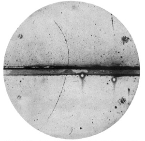
Hace poco fue el aniversario del nacimiento de Paul Dirac; además, en el mismo mes de agosto, pero en 1932 (treinta años más tarde del nacimiento de Dirac), se encontraría evidencia experimental de la existencia del positrón, tan sólo dos años más tarde de que Dirac (auténticamente) lo predijera.
La historia en sí misma es bastante interesante y hay varias lecturas relevantes en la red como ésta o ésta. También está este buenísimo timeline del sitio web del CERN:
Sobre la vida de Dirac también está el famoso libro The Strangest Man de Graham Farmelo, que no he tenido oportunidad de leer porque es complicado conseguirlo en México, aunque en YouTube se encuentra esta charla del mismo Farmelo:
De las relaciones de momento-energía clásicas no-relativista y relativista de una partícula podemos obtener sus ecuaciones mecánico-cuánticas a través de la correspondencia $(E,\vec{p})\to(i\p_t,-i\nabla)$ en unidades naturales ($\hbar=c=1$). En el caso no-relativista, con el potencial $V=V(x,t)$, tenemos que \begin{equation}E=\frac{\vec{p}\cdot\vec{p}}{2m}+V\,\to\,i\p_t=-\frac{\nabla^2}{2m}+\hat{V}\end{equation} que aplicado a una función de onda $\Psi=\Psi(x,t)$, reproduce la ecuación de Schrödinger \begin{equation}i\p_t\Psi=\left(-\frac{\nabla^2}{2m}+\hat{V}\right)\Psi\end{equation} y de manera análoga se puede tomar (el cuadrado de) la relación relativista $E^2=p^2+m^2$ de modo que \begin{equation}\left(-\p_t^2+\nabla^2-m^2\right)\Psi=0\end{equation} que es la ecuación de Klein-Gordon. Finalmente, como se hace con la ecuación de Schödinger, se puede obtener una densidad de probabilidad (que junto con la corriente de probabilidad satisfacen una ecuación de continuidad), que sin embargo para este caso no es positiva definida.
En su artículo The Quantum Theory of the Electron de febrero de 1928, Dirac abordó principalmente este problema para electrones considerando que la ecuación cuántico-relativista debía ser lineal o de primer orden en $\p_t$. Dirac es seguramente uno de los autores de antaño que es más sencillo de leer y su famoso artículo no es la excepción. Resumiendo, Dirac parte de que en relatividad especial la dirección temporal "está al mismo nivel" que las demás, de modo que si la ecuación dinámica es lineal en $\p_t$ (i.e. $p_0$), también tendría que serlo en $\p_i$ (i.e. $p_i$), de donde propone la ecuación de prueba (o ansatz) \begin{equation}\left(p_0+\alpha^ip_i+\beta\right)\Psi=0\end{equation} que debe además ser compatible con la relación de energía-momento relativista, i.e. debe reproducir la ecuación de Klein-Gordon (interpretada como un límite clásico --large quantum numbers) si se eleva al cuadrado el lado izquierdo, de donde obtiene relaciones de las que se sigue que los $\alpha_\mu$ no pueden ser números ordinarios y pueden representarse por matrices. Dirac luego construye un caso particular de estas matrices en lo que hoy conocemos como una representación del álgebra de Clifford. Concretamente, en notación moderna (Dirac la escribe también de forma parecida cuando demuestra que la ecuación es invariante ante transformaciones de Lorentz), \begin{equation}\left(i\gamma^\mu\p_\mu-m\right)\psi=0\end{equation} es la ecuación de Dirac con $\{\gamma^\mu,\gamma^\nu\}=\gamma^\mu\gamma^\nu+\gamma^\nu\gamma^\mu=2\eta^{\mu\nu}\mathbb{I}$ el álgebra de Clifford (Dirac encuentra una representación particular, notando antes que cualquiera debe estár formada por matrices de al menos 4x4) y $\psi$ es un 4-vector, que concretamente en teoría cuántica de campos se conoce como espinor (aunque desde antes se conocía así precisamente por poderse relacionar con el espín de los electrones).
De su ecuación, Dirac resolvió el problema de la densidad de probabilidad negativa [otra forma de determinar los coeficientes de la ecuación de Dirac es precisamente buscando que se satisfaga una ecuación de continuidad de tipo $\p_t(\psi^\dagger\psi)+\nabla\cdot\vec{j}=0$] pero persistía otro problema importante: energías negativas. Resulta que las soluciones de la ecuación de Dirac pueden descomponerse en dos espinores de dos componentes que son eigenestados de energía positiva y negativa. Clásicamente las energías negativas pueden simplemente ignorarse por no tener sentido físico y nada impide descartarlas, de cualquier modo en cuántica estos estados no pueden ignorarse así nada más, ya que la teoría misma requiere tener conjuntos completos (y ortonormales) de eigenestados.
Así pues, Dirac, viendo al monstruo que había creado, atacó también de manera bastante ingeniosa este problema en el artículo A Theory of Electrons and Protons: los electrones son fermiones, así que están sujetos al principio de exclusión de Pauli y por tanto los estados de energía negativa deben estar todos ocupados, siendo accesibles únicamente los de energía positiva. Esto es lo que se conoce como el mar de Dirac. Pero Dirac no se detuvo ahí, notó además que un hueco en el mar de Dirac se comporta como una partícula con carga positiva y el resto de propiedades del electrón: el antielectrón o positrón, que además se aniquila con el electrón emitiendo radiación.
Finalmente el mar de Dirac resultó ser sólo una pifia, de cualquier modo, increíblemente llevó a la respuesta correcta sobre el positrón y luego en general sobre la antimateria. Hoy (y desde algo así como 1934) la ecuación de Dirac únicamente se entiende consistentemente en el contexto de la teoría cuántica de campos: el espinor no es una función de onda, sino un campo clásico que se cuantiza en partículas de espín 1/2 y las antipartículas no están asociadas necesariamente sólo a fermiones, además el Hamiltoniano asociado a la ecuación de Dirac es positivo definido, de modo que es acotado por abajo, como debe, y desaparecen las energías negativas. De manera análoga, más tarde la ecuación de Klein-Gordon fue interpretada por Pauli (?) como una para un campo de espín nulo, también con un Hamiltoniano positivo definido y energías positivas.
In this attempt, the success seems to have been on the side of Dirac rather than logic.
- Pauli sobre Dirac
La predicción de Dirac seguramente era descabellada, además de que nunca se había reportado la observación experimental de algo parecido. Como sea, y contrario a muchas ideas relevantes actualmente, se tenía la ventaja de que se podía falsificar rápidamente su predicción, y así ocurrió con un experimento de Carl Anderson en 1932.
Carl D. Anderson, Physical Review Vol.43, p491 (1933)
Y la idea es bastante simple: utilizar una cámara de niebla: un detector de partículas que funciona mediante vapor de agua supersaturado. El vapor de la cámara de niebla se ioniza cuando cierta radiación ionizante pasa por él, en este caso rayos cósmicos (apenas descubiertos), lo que genera el rastro de un camino ionizado que se fotografía para ser analizado. Si además se aplica un campo magnético, las partículas se curvarán en cierta dirección debido a la fuerza de Lorentz.
Producción de un electrón y un positrón a partir de un fotón de alta energía. Fuente: http://teachers.web.cern.ch
A fin de cuentas Anderson encontró que la partícula que estaba midiendo no podía ser un protón y que correspondía al electrón de carga positiva, que bautizó como positrón. Y el resto es historia, se siguieron descubriendo antipartículas y se generó la noción de la antimateria, que puede ser tan estigmatizada por la cantidad de energía que libera al aniquilarse con la materia hasta ser tan mundana por aplicaciones como la tomografía por emisión de positrones.
When I was a young man, Dirac was my hero. He made a breakthrough, a new method of doing physics. He had the courage to simply guess at the form of an equation, the equation we now call the Dirac equation, and to try to interpret it afterwards. Maxwell in his day got his equations, but only in an enormous mass of 'gear wheels' and so forth.
 738-756")


 que igualmente a primer vista es intimidante pero realmente la idea para reconocerla es la misma que para la identidad de 4 puntos (\ref{Jacobistruct}) y en este caso las permutaciones cíclicas ocurren para los índices que comparten el propagador alrededor del cual se toma la identidad (en este caso $b_1$). En términos de diagramas, uno puede partir de un diagrama en forma multiperiferal (primer diagrama de izquierda a derecha) y luego hacer ambos un intercambio de aristas y una forma de "tenedor-Y" alrededor del propagador en cuestión. Lo del tenedor-Y es relevante porque puede generar diagramas con topologías distintas a la del diagrama original.
")


 sobre el comportamiento UV en gravedad")